Map single cells to Space (Slide-seqV2 Mouse Hippocampus)
This tutorial demonstrates how to map single-cell RNA sequencing (scRNA-seq) data to Slide-seqV2 data of the mouse hippocampus.
[1]:
import os
from time import time

import anndata as ad
import scanpy as sc
from SC2Spa import tl, pp, pl, sva

import pandas as pd

from numpy.random import seed
from tensorflow.random import set_seed
import tensorflow as tf
[2]:
import SC2Spa

print(SC2Spa.__all__)
print('*'*20)
print('Version:', SC2Spa.__version__)
['__title__', '__summary__', '__uri__', '__version__', '__author__', '__email__', '__license__', '__copyright__']
********************
Version: 1.2.3
Download datasets
Download the necessary datasets for the tutorial and saves them in a directory named “Dataset”:
Create the “Dataset” directory if it doesn’t already exist.
Download two AnnData objects (.h5ad files) containing scRNA-seq data and saves them in the “Dataset” directory.
Download a CSV file, likely containing spatial information or metadata for the Slide-seqV2 data, and saves it in the “Dataset” directory.
These downloaded files will be used in the subsequent steps of the tutorial.
[2]:
if not os.path.exists('Dataset'):
    os.makedirs('Dataset')
!wget https://figshare.com/ndownloader/files/38736651 -O Dataset/AdataMH1.h5ad
!wget https://figshare.com/ndownloader/files/38738136 -O Dataset/AMB_HC.h5ad
!wget https://figshare.com/ndownloader/files/38756529 -O Dataset/ssHippo_RCTD.csv
--2023-01-24 19:02:05--  https://figshare.com/ndownloader/files/38736651
Resolving figshare.com (figshare.com)... 52.51.33.13, 54.229.244.39, 2a05:d018:1f4:d003:e01c:5f24:fcad:4854, ...
Connecting to figshare.com (figshare.com)|52.51.33.13|:443... connected.
HTTP request sent, awaiting response... 302 Found
Location: https://s3-eu-west-1.amazonaws.com/pfigshare-u-files/38736651/AdataMH1.h5ad?X-Amz-Algorithm=AWS4-HMAC-SHA256&X-Amz-Credential=AKIAIYCQYOYV5JSSROOA/20230124/eu-west-1/s3/aws4_request&X-Amz-Date=20230124T180205Z&X-Amz-Expires=10&X-Amz-SignedHeaders=host&X-Amz-Signature=707e4f23f121415d52c1dab8b3e707d95df4ac571f540fb86d5be761edda42ab [following]
--2023-01-24 19:02:05--  https://s3-eu-west-1.amazonaws.com/pfigshare-u-files/38736651/AdataMH1.h5ad?X-Amz-Algorithm=AWS4-HMAC-SHA256&X-Amz-Credential=AKIAIYCQYOYV5JSSROOA/20230124/eu-west-1/s3/aws4_request&X-Amz-Date=20230124T180205Z&X-Amz-Expires=10&X-Amz-SignedHeaders=host&X-Amz-Signature=707e4f23f121415d52c1dab8b3e707d95df4ac571f540fb86d5be761edda42ab
Resolving s3-eu-west-1.amazonaws.com (s3-eu-west-1.amazonaws.com)... 52.218.100.35, 52.92.17.88, 52.218.36.194, ...
Connecting to s3-eu-west-1.amazonaws.com (s3-eu-west-1.amazonaws.com)|52.218.100.35|:443... connected.
HTTP request sent, awaiting response... 200 OK
Length: 73481745 (70M) [application/octet-stream]
Saving to: ‘Dataset/AdataMH1.h5ad’

Dataset/AdataMH1.h5 100%[===================>]  70.08M  16.5MB/s    in 4.3s

2023-01-24 19:02:10 (16.4 MB/s) - ‘Dataset/AdataMH1.h5ad’ saved [73481745/73481745]

--2023-01-24 19:02:10--  https://figshare.com/ndownloader/files/38738136
Resolving figshare.com (figshare.com)... 54.229.244.39, 52.51.33.13, 2a05:d018:1f4:d000:a2bd:ffac:4123:16e9, ...
Connecting to figshare.com (figshare.com)|54.229.244.39|:443... connected.
HTTP request sent, awaiting response... 302 Found
Location: https://s3-eu-west-1.amazonaws.com/pfigshare-u-files/38738136/AMB_HC.h5ad?X-Amz-Algorithm=AWS4-HMAC-SHA256&X-Amz-Credential=AKIAIYCQYOYV5JSSROOA/20230124/eu-west-1/s3/aws4_request&X-Amz-Date=20230124T180210Z&X-Amz-Expires=10&X-Amz-SignedHeaders=host&X-Amz-Signature=4e1526450439464860b9e701961f56fe0cc70ca64986c9e4933dfff62cacdbf7 [following]
--2023-01-24 19:02:10--  https://s3-eu-west-1.amazonaws.com/pfigshare-u-files/38738136/AMB_HC.h5ad?X-Amz-Algorithm=AWS4-HMAC-SHA256&X-Amz-Credential=AKIAIYCQYOYV5JSSROOA/20230124/eu-west-1/s3/aws4_request&X-Amz-Date=20230124T180210Z&X-Amz-Expires=10&X-Amz-SignedHeaders=host&X-Amz-Signature=4e1526450439464860b9e701961f56fe0cc70ca64986c9e4933dfff62cacdbf7
Resolving s3-eu-west-1.amazonaws.com (s3-eu-west-1.amazonaws.com)... 52.92.32.96, 52.218.112.179, 52.218.41.251, ...
Connecting to s3-eu-west-1.amazonaws.com (s3-eu-west-1.amazonaws.com)|52.92.32.96|:443... connected.
HTTP request sent, awaiting response... 200 OK
Length: 334743216 (319M) [application/octet-stream]
Saving to: ‘Dataset/AMB_HC.h5ad’

Dataset/AMB_HC.h5ad 100%[===================>] 319.24M  27.1MB/s    in 15s

2023-01-24 19:02:25 (21.5 MB/s) - ‘Dataset/AMB_HC.h5ad’ saved [334743216/334743216]

--2023-01-24 19:02:25--  https://figshare.com/ndownloader/files/38756529
Resolving figshare.com (figshare.com)... 54.229.244.39, 52.51.33.13, 2a05:d018:1f4:d000:a2bd:ffac:4123:16e9, ...
Connecting to figshare.com (figshare.com)|54.229.244.39|:443... connected.
HTTP request sent, awaiting response... 302 Found
Location: https://s3-eu-west-1.amazonaws.com/pfigshare-u-files/38756529/ssHippo_RCTD.csv?X-Amz-Algorithm=AWS4-HMAC-SHA256&X-Amz-Credential=AKIAIYCQYOYV5JSSROOA/20230124/eu-west-1/s3/aws4_request&X-Amz-Date=20230124T180225Z&X-Amz-Expires=10&X-Amz-SignedHeaders=host&X-Amz-Signature=b193bef70a79f0cc0f52f3db99adb8362f86f9b290ca5b5db06e9ff72688dd36 [following]
--2023-01-24 19:02:26--  https://s3-eu-west-1.amazonaws.com/pfigshare-u-files/38756529/ssHippo_RCTD.csv?X-Amz-Algorithm=AWS4-HMAC-SHA256&X-Amz-Credential=AKIAIYCQYOYV5JSSROOA/20230124/eu-west-1/s3/aws4_request&X-Amz-Date=20230124T180225Z&X-Amz-Expires=10&X-Amz-SignedHeaders=host&X-Amz-Signature=b193bef70a79f0cc0f52f3db99adb8362f86f9b290ca5b5db06e9ff72688dd36
Resolving s3-eu-west-1.amazonaws.com (s3-eu-west-1.amazonaws.com)... 52.218.101.235, 52.218.101.51, 52.218.60.75, ...
Connecting to s3-eu-west-1.amazonaws.com (s3-eu-west-1.amazonaws.com)|52.218.101.235|:443... connected.
HTTP request sent, awaiting response... 200 OK
Length: 1357460 (1.3M) [text/csv]
Saving to: ‘Dataset/ssHippo_RCTD.csv’

Dataset/ssHippo_RCT 100%[===================>]   1.29M  5.18MB/s    in 0.2s

2023-01-24 19:02:26 (5.18 MB/s) - ‘Dataset/ssHippo_RCTD.csv’ saved [1357460/1357460]
[3]:
if not os.path.exists('tutorial1'):
    os.makedirs('tutorial1')
#%cd tutorial1
Data Preparation for Spatial Transcriptomics Analysis
1. Load Data
First, we load the reference and query datasets stored in AnnData objects:
Reference dataset: Slide-seqV2 data
Query dataset: scRNA-seq data
This involves reading .h5ad files that contain the data.
2. Standardize Gene Names
To ensure consistency in our datasets:
Convert all gene names to uppercase (Optional)
Ensure all gene names are unique within each dataset
3. Normalize the Data
Normalization is crucial for scRNA-seq data processing:
Normalize so each cell has a total count of 10,000
Log-transform the data
This mitigates the effects of varying sequencing depths across cells
4. Load and Integrate Annotations (Specific for the tutorial data)
Annotations provide additional metadata about the cells:
Load annotations from a CSV file
Integrate with our reference (Slide-seqV2) dataset
Merge cell type information
Add spatial coordinates to the dataset
5. Clean and Simplify Annotations (Specific for the tutorial data)
For the query (scRNA-seq) dataset:
Clean and simplify cell type names
Ensure consistency and readability
Remove unnecessary characters
Standardize naming conventions
With these steps completed, our reference and query datasets are loaded, normalized, and annotated, ready for further analysis. Subsequent sections of this tutorial will explore various downstream analyses and visualizations.
[4]:
#Load
adata_ref = ad.read_h5ad('Dataset/AdataMH1.h5ad')
adata_query = ad.read_h5ad('Dataset/AMB_HC.h5ad')

adata_ref.var_names = adata_ref.var_names.str.upper()
adata_query.var_names = adata_query.var_names.str.upper()

adata_ref.var_names_make_unique()
adata_query.var_names_make_unique()

#Normalize
sc.pp.normalize_total(adata_ref, target_sum=1e4)
sc.pp.log1p(adata_ref)
sc.pp.normalize_total(adata_query, target_sum=1e4)
sc.pp.log1p(adata_query)

#Load annotation
Anno = pd.read_csv('Dataset/ssHippo_RCTD.csv', index_col = 0)
Anno['MCT'] = 't'
index1 = Anno.index[(Anno['celltype_1'] == Anno['celltype_2'])]
Anno['MCT'][index1] = Anno['celltype_1'][index1]
index2 = Anno.index[(Anno['celltype_1'] != Anno['celltype_2'])]
Anno['MCT'][index2] = (Anno['celltype_1'][index2] + '_' + Anno['celltype_2'][index2]).apply(lambda x: '_'.join(sorted(set(x.split('_')))))
adata_ref.obs = adata_ref.obs.merge(Anno, left_index = True, right_index = True, how = 'left')

adata_ref.obsm['spatial'] = adata_ref.obs[['xcoord', 'ycoord']].values


adata_query.obs['common_name'] = adata_query.obs['common_name'].str.replace('?', '')
adata_query.obs['simp_name'] = adata_query.obs['common_name'].str.split('.',
                        expand = True)[0].str.split(',', expand = True)[0].str.split(' \(',
                                    expand = True)[0].str.replace('cortexm', 'cortex').replace('Medial entorrhinal cortex', 'Medial entorhinal cortex')
/home/linbuliao/anaconda3/lib/python3.10/site-packages/anndata/_core/anndata.py:1832: UserWarning: Variable names are not unique. To make them unique, call `.var_names_make_unique`.
  utils.warn_names_duplicates("var")
/tmp/ipykernel_1954104/2707152110.py:30: FutureWarning: The default value of regex will change from True to False in a future version. In addition, single character regular expressions will *not* be treated as literal strings when regex=True.
  adata_query.obs['common_name'] = adata_query.obs['common_name'].str.replace('?', '')
Select genes using Wasserstein distance (Optional)
This step is time-consuming on Slide-seqV2 data
In this section, we will download the precalculated Wasserstein distances between the scRNA-seq and Slide-seqV2 (ST) datasets. Then, we will filter the genes based on a specified cutoff value for the Wasserstein distance. # ### 1. Set Parameters First, we define the root directory where the files will be saved, a cutoff value for filtering the Wasserstein distances, and the filename for the downloaded data.
2. Download Precalculated Wasserstein Distances
We then download the CSV file containing the precalculated Wasserstein distances. This file compares the distances between the scRNA-seq and Slide-seqV2 (ST) datasets. The file is saved in the specified directory.
3. Load and Filter the Data
After downloading, we load the CSV file into a pandas dataframe. We then filter the genes based on the specified cutoff value for the Wasserstein distance. Only genes with a distance less than the cutoff value are selected.
By following these steps, we have downloaded the necessary data and filtered the genes based on their Wasserstein distances. This prepares us for further analysis and visualization in the subsequent sections of this tutorial.
[ ]:
'''
sta = time()
JGs, WDs = tl.WassersteinD(adata_ref, adata_query, sparse = True,
                           WD_cutoff = 0.1, root = 'WDs/', save = 'WDs_T2')

end = time()
print((end - sta) / 60.0, 'min')
'''
[5]:
'''
root = 'WDs/'
'''

WD_cutoff = 0.4
root = 'tutorial1/'
save = 'WDs_T2'

# Download the precalculated Wasserstain distances between the scRNA-seq and ST datasets.
!wget https://figshare.com/ndownloader/files/38938874 -O tutorial1/WDs_T2.csv

WDs = pd.read_csv(root + save + '.csv')
JGs = sorted(WDs[WDs['Wasserstein_Distance'] < WD_cutoff]['Gene'].tolist())
--2023-07-31 18:33:58--  https://figshare.com/ndownloader/files/38938874
Resolving figshare.com (figshare.com)... 34.240.187.105, 34.255.145.108, 2a05:d018:1f4:d003:d9a0:7d81:fa75:f690, ...
Connecting to figshare.com (figshare.com)|34.240.187.105|:443... connected.
HTTP request sent, awaiting response... 302 Found
Location: https://s3-eu-west-1.amazonaws.com/pfigshare-u-files/38938874/WDs_T2.csv?X-Amz-Algorithm=AWS4-HMAC-SHA256&X-Amz-Credential=AKIAIYCQYOYV5JSSROOA/20230731/eu-west-1/s3/aws4_request&X-Amz-Date=20230731T163358Z&X-Amz-Expires=10&X-Amz-SignedHeaders=host&X-Amz-Signature=185a094c4c63d1153e36fb8109aa240d382f02e088ef07ea62e48b45d938f86e [following]
--2023-07-31 18:33:58--  https://s3-eu-west-1.amazonaws.com/pfigshare-u-files/38938874/WDs_T2.csv?X-Amz-Algorithm=AWS4-HMAC-SHA256&X-Amz-Credential=AKIAIYCQYOYV5JSSROOA/20230731/eu-west-1/s3/aws4_request&X-Amz-Date=20230731T163358Z&X-Amz-Expires=10&X-Amz-SignedHeaders=host&X-Amz-Signature=185a094c4c63d1153e36fb8109aa240d382f02e088ef07ea62e48b45d938f86e
Resolving s3-eu-west-1.amazonaws.com (s3-eu-west-1.amazonaws.com)... 52.218.44.200, 52.92.0.192, 52.92.34.120, ...
Connecting to s3-eu-west-1.amazonaws.com (s3-eu-west-1.amazonaws.com)|52.218.44.200|:443... connected.
HTTP request sent, awaiting response... 200 OK
Length: 562050 (549K) [text/csv]
Saving to: ‘tutorial1/WDs_T2.csv’

tutorial1/WDs_T2.cs 100%[===================>] 548.88K  3.51MB/s    in 0.2s

2023-07-31 18:33:58 (3.51 MB/s) - ‘tutorial1/WDs_T2.csv’ saved [562050/562050]
Fine Mapping
Train SC2Spa with the genes selected based on Wassertain distance
[8]:
#Download Pretrained Model
!wget https://figshare.com/ndownloader/files/38938871 -O tutorial1/SI_T2_WD.h5
--2023-03-13 13:37:08--  https://figshare.com/ndownloader/files/38938871
Resolving figshare.com (figshare.com)... 54.194.194.40, 63.35.25.157, 2a05:d018:1f4:d000:f9b:6c1a:bd62:eb42, ...
Connecting to figshare.com (figshare.com)|54.194.194.40|:443... connected.
HTTP request sent, awaiting response... 302 Found
Location: https://s3-eu-west-1.amazonaws.com/pfigshare-u-tempfiles/38938871/SI_T2_WD.h5?X-Amz-Algorithm=AWS4-HMAC-SHA256&X-Amz-Credential=AKIAIYCQYOYV5JSSROOA/20230313/eu-west-1/s3/aws4_request&X-Amz-Date=20230313T123708Z&X-Amz-Expires=10&X-Amz-SignedHeaders=host&X-Amz-Signature=d606a69fad03d628111274b12094cadca3282430cd772e704fa7846523e6d184 [following]
--2023-03-13 13:37:08--  https://s3-eu-west-1.amazonaws.com/pfigshare-u-tempfiles/38938871/SI_T2_WD.h5?X-Amz-Algorithm=AWS4-HMAC-SHA256&X-Amz-Credential=AKIAIYCQYOYV5JSSROOA/20230313/eu-west-1/s3/aws4_request&X-Amz-Date=20230313T123708Z&X-Amz-Expires=10&X-Amz-SignedHeaders=host&X-Amz-Signature=d606a69fad03d628111274b12094cadca3282430cd772e704fa7846523e6d184
Resolving s3-eu-west-1.amazonaws.com (s3-eu-west-1.amazonaws.com)... 52.218.90.35, 52.218.120.16, 52.218.88.11, ...
Connecting to s3-eu-west-1.amazonaws.com (s3-eu-west-1.amazonaws.com)|52.218.90.35|:443... connected.
HTTP request sent, awaiting response... 200 OK
Length: 1016306424 (969M) [application/octet-stream]
Saving to: ‘tutorial1/SI_T2_WD.h5’

tutorial1/SI_T2_WD. 100%[===================>] 969.22M  21.7MB/s    in 46s

2023-03-13 13:37:55 (21.1 MB/s) - ‘tutorial1/SI_T2_WD.h5’ saved [1016306424/1016306424]
[6]:
#Set random generator seed
seed_num = 2023
seed(seed_num)
set_seed(seed_num)
tf.keras.utils.set_random_seed(seed_num)

'''
Finely map single cells to spatial locations.
A model will be trained and saved to `root+name+'.h5'` if model_path is None and save is True.
The predicted coordinates of single cells will be saved in adata_query.obsm['spatial_mapping']
The predicted coordinates of beads will be saved in adata_ref.obsm['spatial_mapping']
Fine mapping information will be saved in adata_ref.obs['FM'] and adata_query.obs['FM']. True if a cell/bead
was mapped, otherwise False.
'''

'''
sta = time()

neighbors, dis = tl.FineMapping(adata_ref, adata_query, sparse =True, JGs = None,
                                model_path = None, root = 'Model_SI/',
                                name = 'SI_T2', l1_reg = 1e-5, l2_reg = 0, dropout = 0.05, epoch = 500,
                                batch_size = 4096, nodes = [4096, 1024, 256, 64, 16, 4], lrr_patience = 20,
                                ES_patience = 50, min_lr = 1e-5, save = True, polar = True,
                                n_neighbors = 1000, dis_cutoff = 20, seed = seed_num)

end = time()
print((end - sta) / 60.0, 'min')
'''

tl.FineMapping(adata_ref, adata_query, JGs = JGs, sparse =True,
               model_path = 'tutorial1/SI_T2_WD.h5', polar = True,
               n_layer_cell = [1, 4], cell_radius = 5,
               n_neighbors = 1000, dis_cutoff = 15, seed = seed_num)
n of Referece Genes: 20527
n of Target Genes: 24509
n of Selected Genes: 19577
(35349, 19577)
(127165, 19577)
2023-07-31 18:35:03.400837: W tensorflow/core/framework/cpu_allocator_impl.cc:82] Allocation of 320749568 exceeds 10% of free system memory.
2023-07-31 18:35:03.762507: W tensorflow/core/framework/cpu_allocator_impl.cc:82] Allocation of 4698480000 exceeds 10% of free system memory.
2023-07-31 18:35:08.850605: W tensorflow/core/framework/cpu_allocator_impl.cc:82] Allocation of 4698480000 exceeds 10% of free system memory.
2023-07-31 18:35:22.227028: W tensorflow/core/framework/cpu_allocator_impl.cc:82] Allocation of 4698480000 exceeds 10% of free system memory.
2023-07-31 18:35:27.846322: W tensorflow/core/framework/cpu_allocator_impl.cc:82] Allocation of 4698480000 exceeds 10% of free system memory.
[7]:
print(adata_query.shape)
print(adata_query.obs['FM'].sum())
print(adata_query.obs['Recon_scST'].sum())
(127165, 24509)
91395
50305
[8]:
# Distribution of the number of cells assigned to ST beads
ST_beads_n_cells = adata_query.obs[adata_query.obs['Recon_scST']].groupby('ClosestBead_name').sum()['Recon_scST']
print(ST_beads_n_cells.value_counts())
ST_beads_n_cells.hist()
/tmp/ipykernel_1954104/3032249390.py:2: FutureWarning: The default value of numeric_only in DataFrameGroupBy.sum is deprecated. In a future version, numeric_only will default to False. Either specify numeric_only or select only columns which should be valid for the function.
  ST_beads_n_cells = adata_query.obs[adata_query.obs['Recon_scST']].groupby('ClosestBead_name').sum()['Recon_scST']
1    7435
2    5375
3    4160
4    3045
5    1492
Name: Recon_scST, dtype: int64
[8]:
<Axes: >

[9]:
layer = 0
print(adata_query.obs[adata_query.obs['Recon_scST_layer'] == layer]['Dis2ClosestBead'].mean())
adata_query.obs[adata_query.obs['Recon_scST_layer'] == layer]['Dis2ClosestBead'].hist()
3.2041114390688876
[9]:
<Axes: >

[10]:
layer = 1
print(adata_query.obs[adata_query.obs['Recon_scST_layer'] == layer]['Dis2ClosestBead'].mean())
adata_query.obs[adata_query.obs['Recon_scST_layer'] == layer]['Dis2ClosestBead'].hist()
9.549904097512195
[10]:
<Axes: >

[11]:
help(tl.FineMapping)
Help on function FineMapping in module SC2Spa.tl:

FineMapping(adata_ref, adata_query, sparse=True, model_path=None, WD_cutoff=None, JGs=None, root='Model_SI/', name='SI', l1_reg=1e-05, l2_reg=0, dropout=0.05, epoch=500, batch_size=4096, nodes=[4096, 1024, 256, 64, 16, 4], lrr_patience=20, ES_patience=50, min_lr=1e-05, save=True, polar=True, FM=True, n_layer_cell=[1, 4], cell_radius=5, n_neighbors=1000, dis_cutoff=15, seed=2023)
    Finely map single cells to spatial locations and Reconstruct ST data at single cell resolution

    1. Finely map single cells to spatial locations.
    A model will be trained and saved to `root+name+'.h5'` if model_path is None and save is True.
    The predicted coordinates of single cells will be saved in adata_query.obsm['spatial_mapping']
    The predicted coordinates of beads will be saved in adata_ref.obsm['spatial_mapping']
    Fine mapping information will be saved in adata_ref.obs['FM'] and adata_query.obs['FM']. True if a cell/bead
    was mapped, otherwise False.

    2. Reconstruct ST data at single cell resolution
    adata_query.obs['Dis2CloestBead'] stores the distance between a cell and the ST bead closest to it
    adata_query.obs['Recon_scST'] marks the cells that are used to reconstruct single-cell ST data
    adata_query.obs['Recon_scST_layer'] stores which reconstruction layer of cells. -1 means
    a cell is not assigned to any ST bead. 0 means a cell is among the closest cells to a ST bead.
    The greater the layer number, the further a cell is to the center of a ST bead.

    Parameters
    ----------
    adata_ref
        Reference anndata object. Gene expression matrix should be the shape of (cell, gene).
        Spatial information should be stored in adata_ref.obsm['spatial'] in `np.array` format
    adata_query
        Query anndata object. Gene expression matrix should be the shape of (cell, gene).
    sparse
        if gene expression is saved in sparse format
    model_path
        The path of a trained model. If not None, parameters for training will be ignored.
    WD_cutoff
        genes with Wasserstein distance lower than the cutoff will be used for mapping
    JGs
        List of genes used for training
    root
        the root path to save the model
    name
        the name used to save the model
    l1_reg
        l1 regularization factor
    l2_reg
        l2 regularization factor
    nodes
        a list that contains the numbers of the nodes of hidden layers
    lrr_patience
        The patience for learning rate reduction
    min_lr
        minimum learning rate
    ES_patience
        The patience for early stopping
    n_neighbors
        Number of the nearest neighbors of a bead or cell. This parameter is for
        the KNN algorithm
    dis_cutoff
        Limit for the distance between a single cell and a ST bead. In the process
         of fine mapping. Only the cells within the cutoff will be retained.
    FM
        Perform fine mapping and reconstruct ST data at single cell resolution if True
    n_layer_cell
        Number of cells in layers for sampling single cells for a ST bead.
    cell_radius
        Radius of a cell. For example, n_layer_cell=[1, 4] and cell_radius=5 means sampling 1 cell
         from cells within 5 to a bead and at most 4 cells from cells between 5 and 15 to the bead.
         It is at most 4 cells because a cell can be sampled more than once to deal with the case
         that a bead has fewer cells than the user specified.
    seed
        seed for reconstructing the single-cell ST data
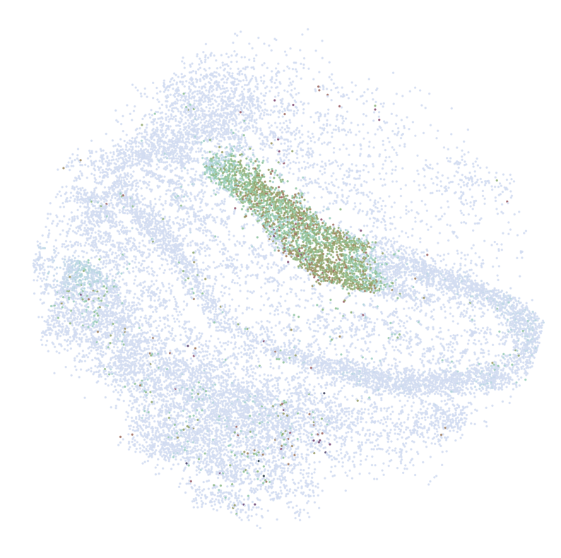
Visualization
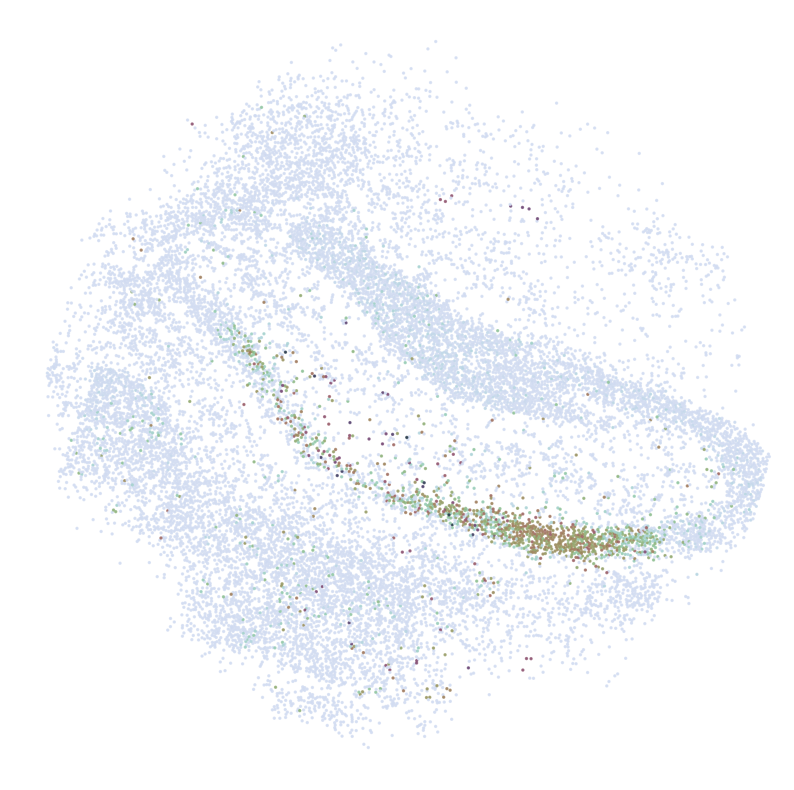
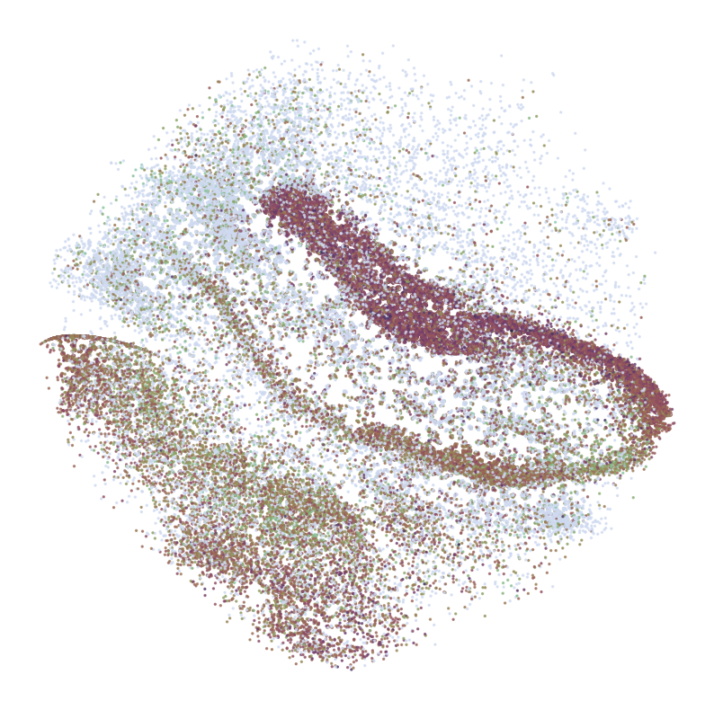
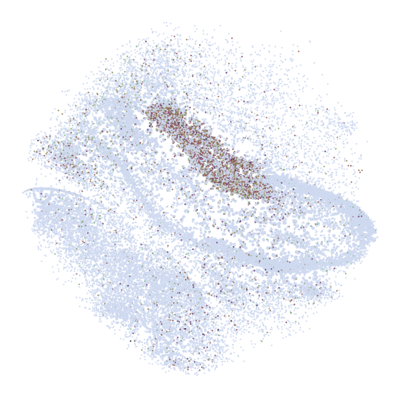
Draw Fine mapping result
[12]:
#for CT in adata_query.obs['simp_name'].unique():
CT_list = ['CA1 Principal cells',
           'CA2 Principal cells',
           'CA3 Principal cells',
           'Dentate Principal cells']
for CT in CT_list:
    print('*'*16)
    print(CT)
    print('*'*16)
    print('Transfer:')
    pl.DrawCT1(adata_query, coords_name = 'spatial_mapping',
                CT = CT, c_name = 'simp_name', FM = True, scST = False,
                root = 'tutorial1/Transfer2/FM_Valid2/', save = 'SC2HC1')
****************
CA1 Principal cells
****************
Transfer:
****************
CA2 Principal cells
****************
Transfer:
****************
CA3 Principal cells
****************
Transfer:
****************
Dentate Principal cells
****************
Transfer:

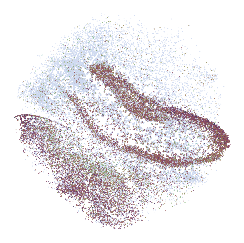
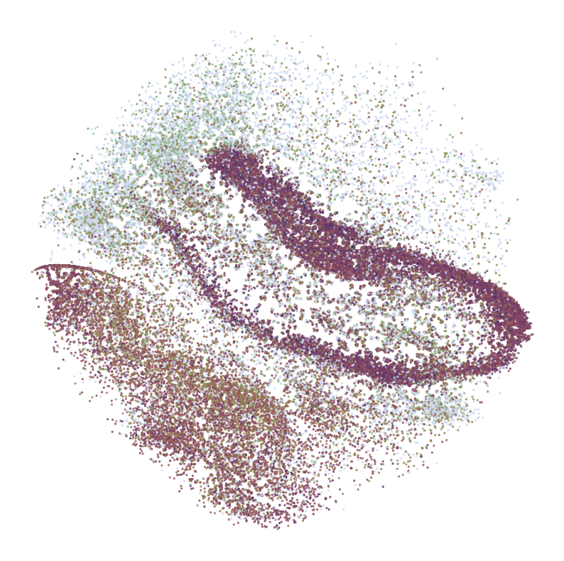
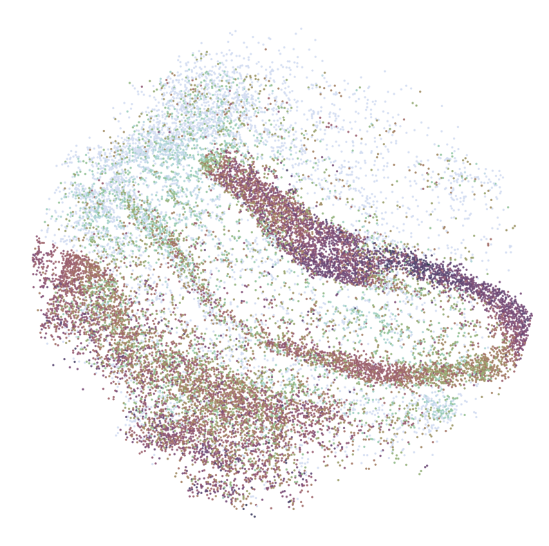
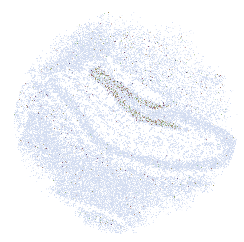
Draw Reconstructed single-cell ST data
[13]:
CT_list = ['CA1 Principal cells',
           'CA2 Principal cells',
           'CA3 Principal cells',
           'Dentate Principal cells']

for CT in CT_list:
    print('*'*16)
    print(CT)
    print('*'*16)
    print('Transfer:')
    pl.DrawCT1(adata_query, coords_name = 'spatial_mapping',
                CT = CT, c_name = 'simp_name', FM = False, scST = True,
                root = 'tutorial1/Transfer2/FM_Valid2/', save = 'SC2HC1')
****************
CA1 Principal cells
****************
Transfer:

****************
CA2 Principal cells
****************
Transfer:

****************
CA3 Principal cells
****************
Transfer:
****************
Dentate Principal cells
****************
Transfer:
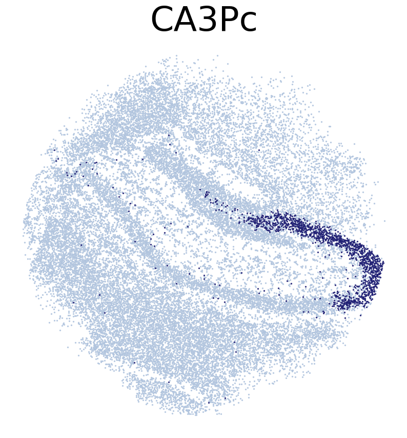
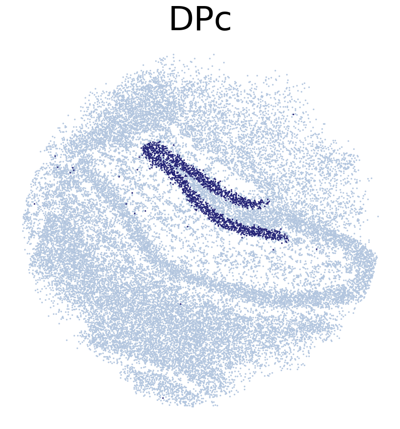
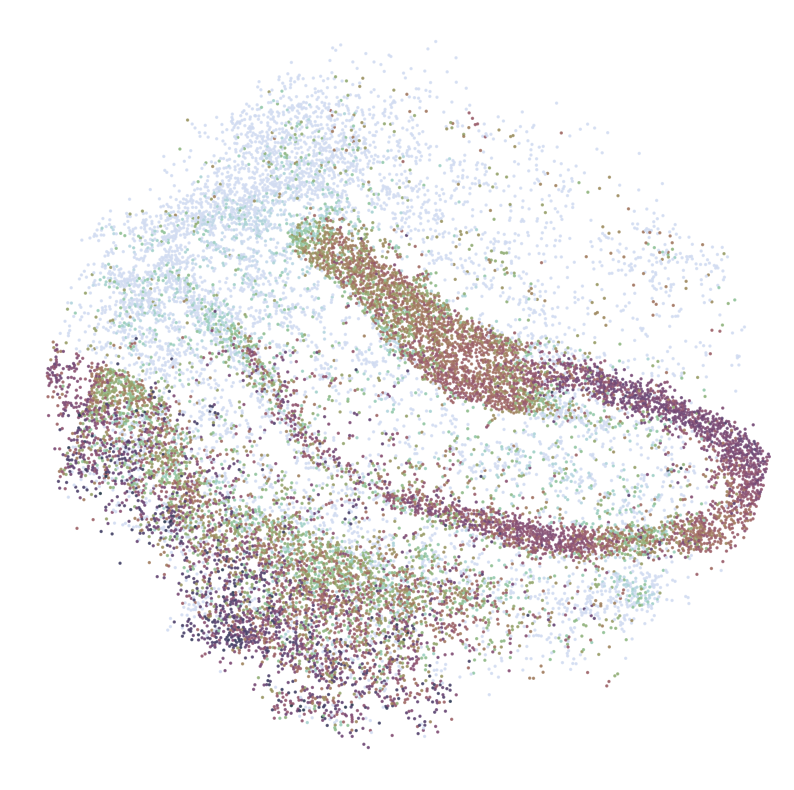
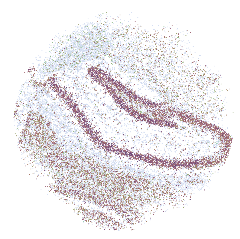
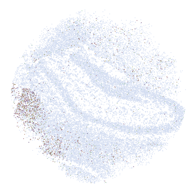
Draw reference ST data
[14]:
CT_list = ['CA1Pc',
           'CA3Pc',
           'DPc']

for CT in CT_list:
    print('*'*16)
    print(CT)
    print('*'*16)
    print('Transfer:')
    pl.DrawCT1(adata_ref, coords_name = 'spatial',
                CT = CT, FM = True, scST = False, c_name = 'SSV2',
                root = 'tutorial1/Transfer2/FM_Valid2/', save = 'HC1')
****************
CA1Pc
****************
Transfer:

****************
CA3Pc
****************
Transfer:
****************
DPc
****************
Transfer:
Train SC2Spa with the shared genes of the single-cell and spatial transcriptomic data
[14]:
#Download Pretrained Model
!wget https://figshare.com/ndownloader/files/38940521 -O tutorial1/SI_T2.h5
--2023-01-24 19:34:28--  https://figshare.com/ndownloader/files/38940521
Resolving figshare.com (figshare.com)... 54.229.244.39, 52.51.33.13, 2a05:d018:1f4:d000:a2bd:ffac:4123:16e9, ...
Connecting to figshare.com (figshare.com)|54.229.244.39|:443... connected.
HTTP request sent, awaiting response... 302 Found
Location: https://s3-eu-west-1.amazonaws.com/pfigshare-u-files/38940521/SI_T2.h5?X-Amz-Algorithm=AWS4-HMAC-SHA256&X-Amz-Credential=AKIAIYCQYOYV5JSSROOA/20230124/eu-west-1/s3/aws4_request&X-Amz-Date=20230124T183428Z&X-Amz-Expires=10&X-Amz-SignedHeaders=host&X-Amz-Signature=f0088c8e6d73948f9c2bf9e6f8ebb311c3398b5d4b4ce396c540c04783237828 [following]
--2023-01-24 19:34:28--  https://s3-eu-west-1.amazonaws.com/pfigshare-u-files/38940521/SI_T2.h5?X-Amz-Algorithm=AWS4-HMAC-SHA256&X-Amz-Credential=AKIAIYCQYOYV5JSSROOA/20230124/eu-west-1/s3/aws4_request&X-Amz-Date=20230124T183428Z&X-Amz-Expires=10&X-Amz-SignedHeaders=host&X-Amz-Signature=f0088c8e6d73948f9c2bf9e6f8ebb311c3398b5d4b4ce396c540c04783237828
Resolving s3-eu-west-1.amazonaws.com (s3-eu-west-1.amazonaws.com)... 52.218.104.234, 52.218.108.19, 52.218.60.35, ...
Connecting to s3-eu-west-1.amazonaws.com (s3-eu-west-1.amazonaws.com)|52.218.104.234|:443... connected.
HTTP request sent, awaiting response... 200 OK
Length: 1036409592 (988M) [application/octet-stream]
Saving to: ‘SI_T2.h5’

SI_T2.h5            100%[===================>] 988.40M  30.3MB/s    in 38s

2023-01-24 19:35:06 (26.2 MB/s) - ‘SI_T2.h5’ saved [1036409592/1036409592]
[15]:
#Set random generator seed
seed_num = 2022
seed(seed_num)
set_seed(seed_num)
tf.keras.utils.set_random_seed(seed_num)

tl.FineMapping(adata_ref, adata_query, JGs = None, sparse =True,
                model_path = 'tutorial1/SI_T2.h5', polar = True,
                n_layer_cell = [1, 4], cell_radius = 5,
                n_neighbors = 1000, dis_cutoff = 15, seed = seed_num)
n of Referece Genes: 20527
n of Target Genes: 24509
n of Selected Genes: 19986
(35349, 19986)
(127165, 19986)
[16]:
print(adata_query.shape)
print(adata_query.obs['FM'].sum())
print(adata_query.obs['Recon_scST'].sum())
(127165, 24509)
87791
42853
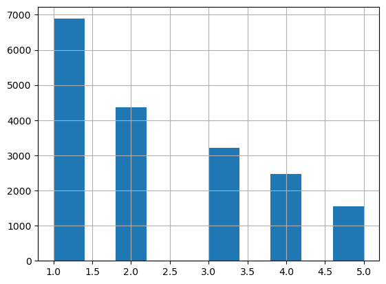
[17]:
# Distribution of the number of cells assigned to ST beads
ST_beads_n_cells = adata_query.obs[adata_query.obs['Recon_scST']].groupby('ClosestBead_name').sum()['Recon_scST']
print(ST_beads_n_cells.value_counts())
ST_beads_n_cells.hist()
1    6885
2    4375
3    3212
4    2468
5    1542
Name: Recon_scST, dtype: int64
/tmp/ipykernel_1954104/3032249390.py:2: FutureWarning: The default value of numeric_only in DataFrameGroupBy.sum is deprecated. In a future version, numeric_only will default to False. Either specify numeric_only or select only columns which should be valid for the function.
  ST_beads_n_cells = adata_query.obs[adata_query.obs['Recon_scST']].groupby('ClosestBead_name').sum()['Recon_scST']
[17]:
<Axes: >
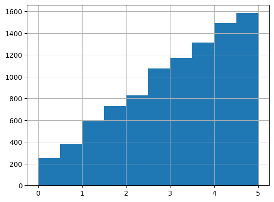
[18]:
layer = 0
print(adata_query.obs[adata_query.obs['Recon_scST_layer'] == layer]['Dis2ClosestBead'].mean())
adata_query.obs[adata_query.obs['Recon_scST_layer'] == layer]['Dis2ClosestBead'].hist()
3.16555484581436
[18]:
<Axes: >
[19]:
layer = 1
print(adata_query.obs[adata_query.obs['Recon_scST_layer'] == layer]['Dis2ClosestBead'].mean())
adata_query.obs[adata_query.obs['Recon_scST_layer'] == layer]['Dis2ClosestBead'].hist()
9.559654472244034
[19]:
<Axes: >

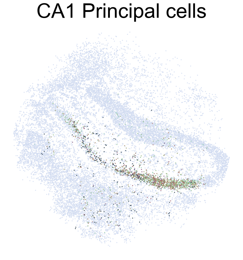
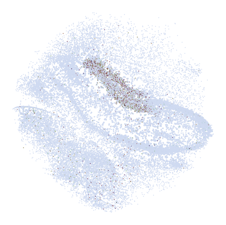
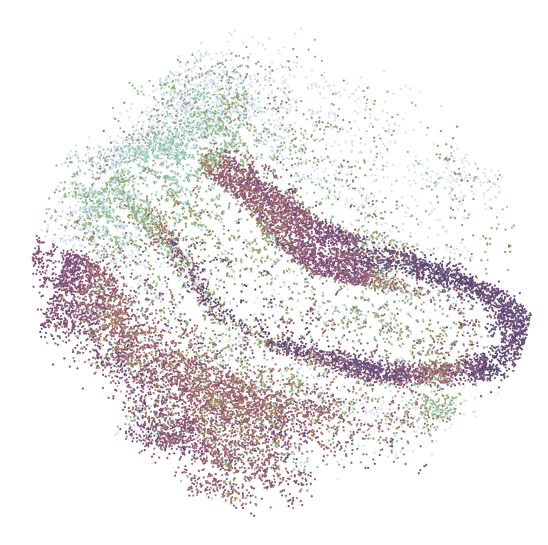
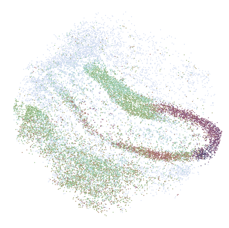
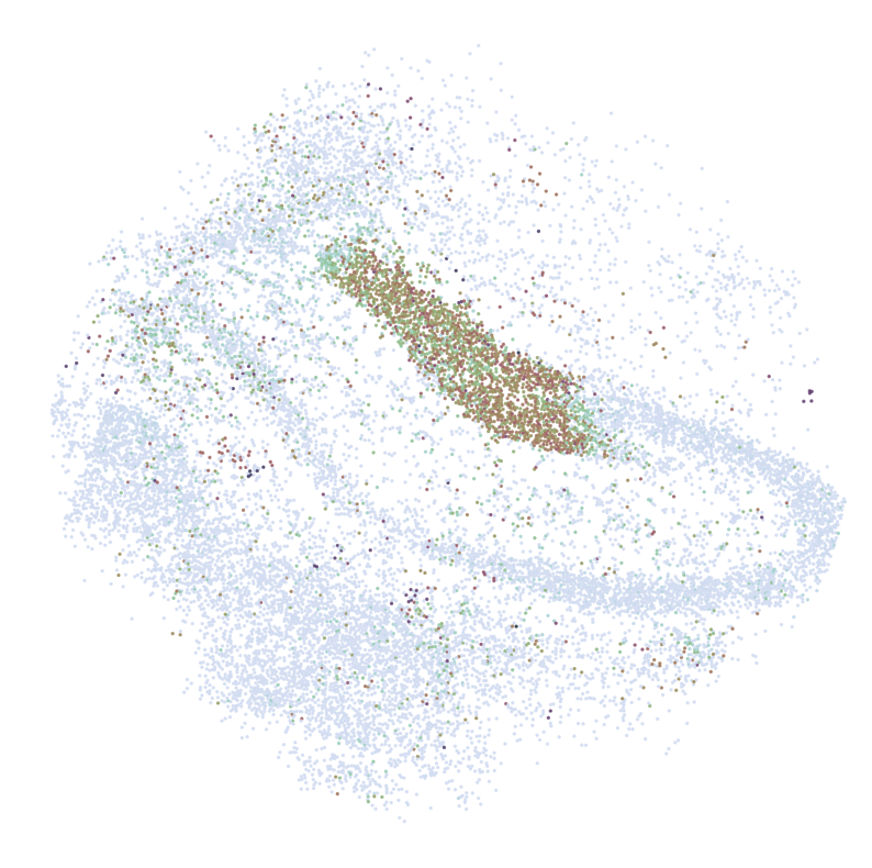
Visualization
Draw Fine mapping result
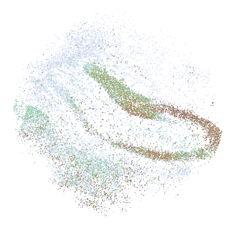
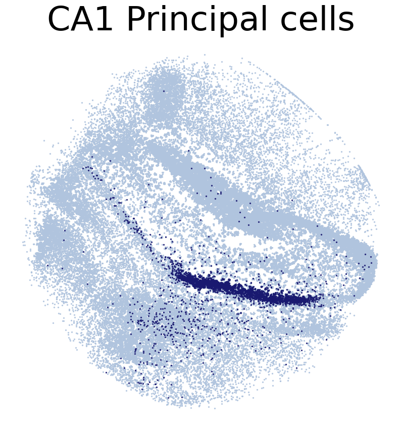
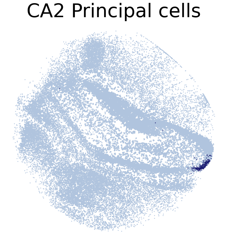
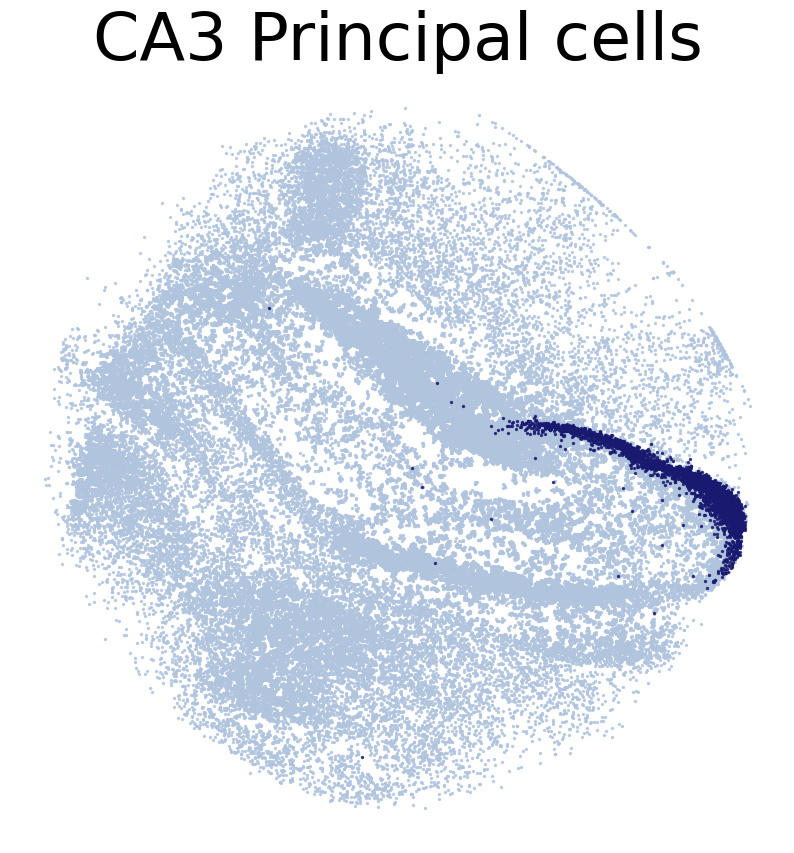
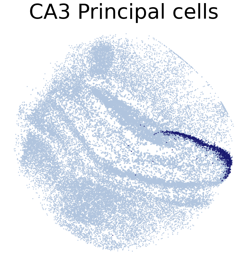
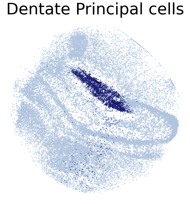
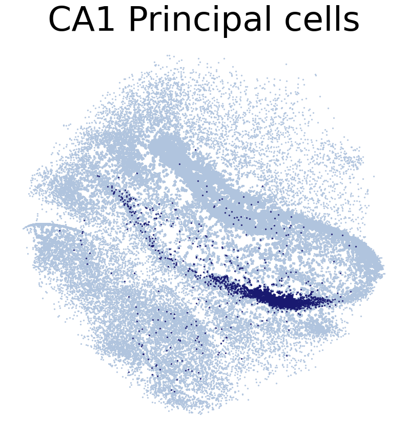
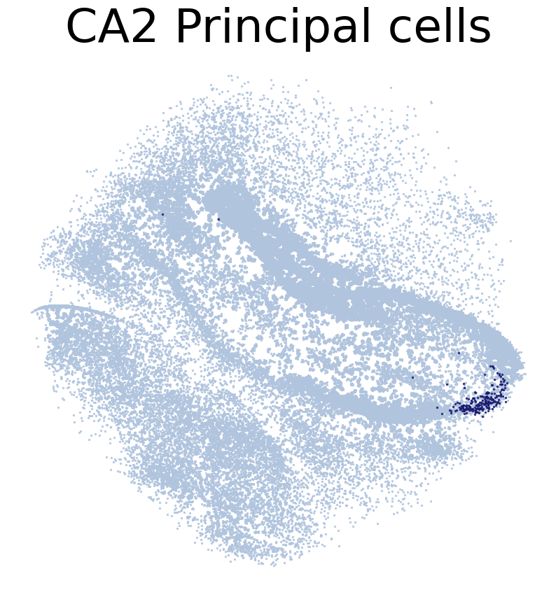
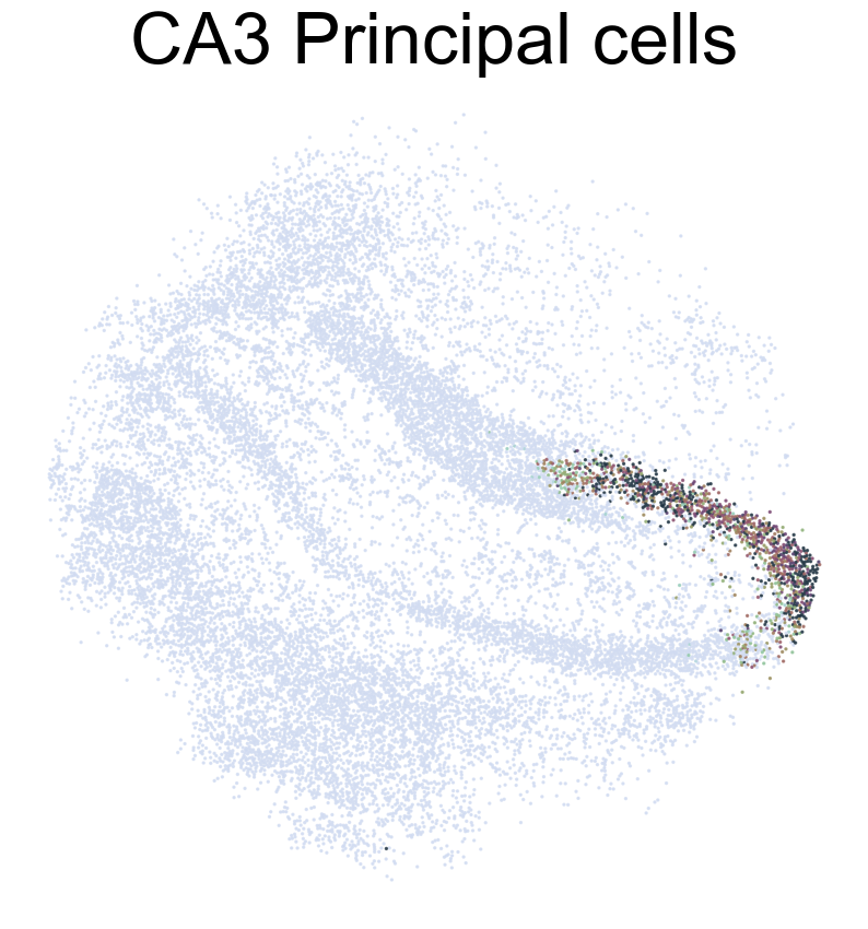
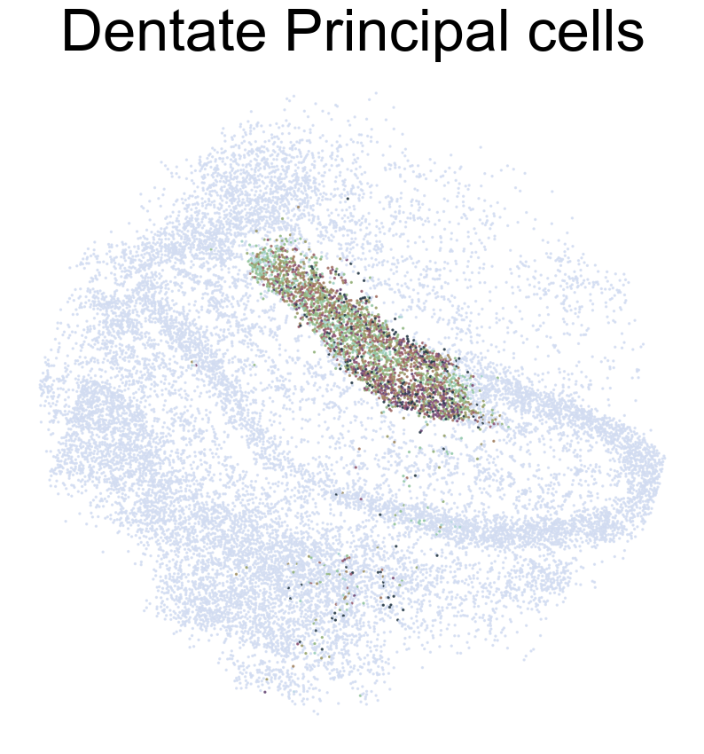
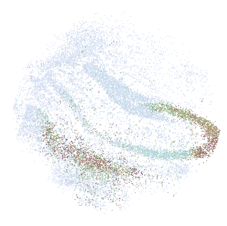
[20]:
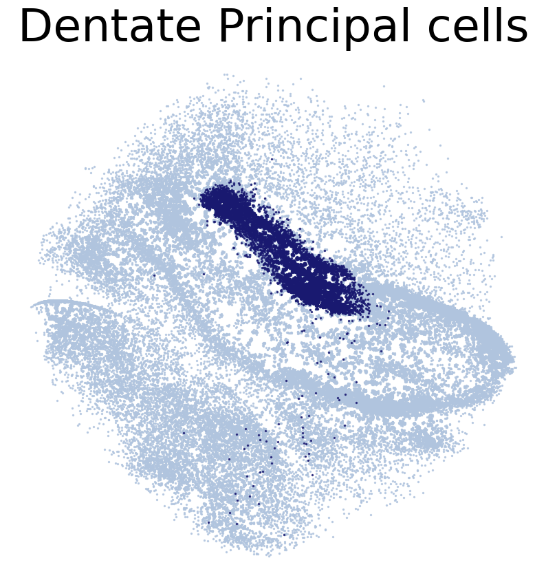
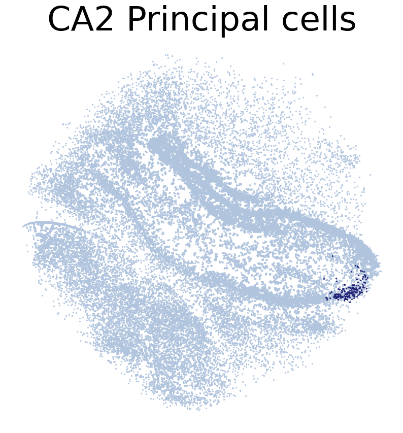
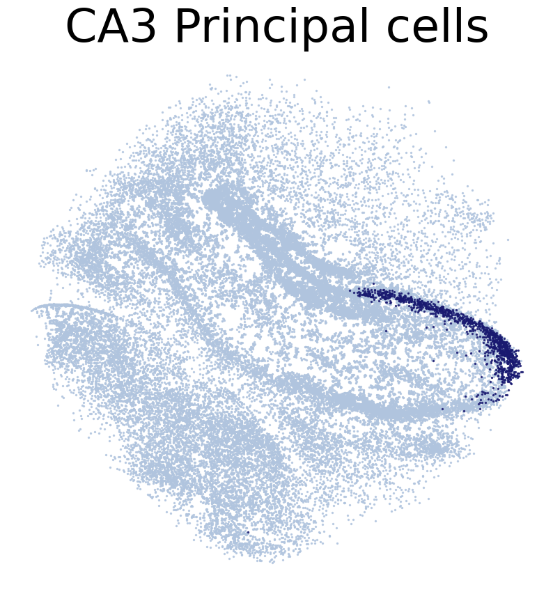
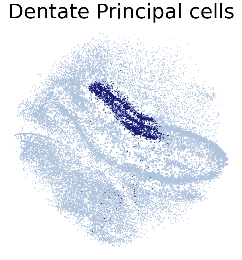
# Location of single cells predicted by SC2Spa

#for CT in adata_query.obs['simp_name'].unique():
CT_list = ['CA1 Principal cells',
           'CA2 Principal cells',
           'CA3 Principal cells',
           'Dentate Principal cells']
for CT in CT_list:
    print('*'*16)
    print(CT)
    print('*'*16)
    print('Transfer:')
    pl.DrawCT1(adata_query, coords_name = 'spatial_mapping',
                CT = CT, c_name = 'simp_name', FM = True, scST = False,
                root = 'tutorial1/Transfer2/FM_Valid2/', save = 'SC2HC1')
****************
CA1 Principal cells
****************
Transfer:
****************
CA2 Principal cells
****************
Transfer:
****************
CA3 Principal cells
****************
Transfer:

****************
Dentate Principal cells
****************
Transfer:
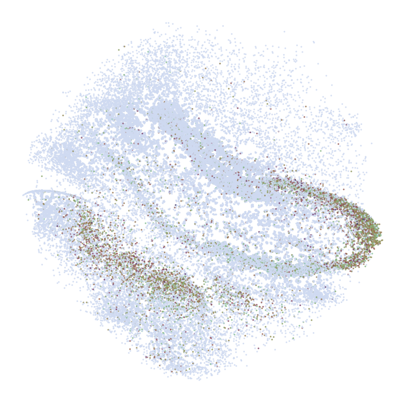
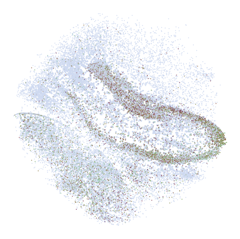
Draw reconstructed single-cell ST data
[21]:
CT_list = ['CA1 Principal cells',
           'CA2 Principal cells',
           'CA3 Principal cells',
           'Dentate Principal cells']

for CT in CT_list:
    print('*'*16)
    print(CT)
    print('*'*16)
    print('Transfer:')
    pl.DrawCT1(adata_query, coords_name = 'spatial_mapping',
                CT = CT, c_name = 'simp_name', FM = False, scST = True,
                root = 'tutorial1/Transfer2/FM_Valid2/', save = 'SC2HC1')
****************
CA1 Principal cells
****************
Transfer:

****************
CA2 Principal cells
****************
Transfer:
****************
CA3 Principal cells
****************
Transfer:
****************
Dentate Principal cells
****************
Transfer:
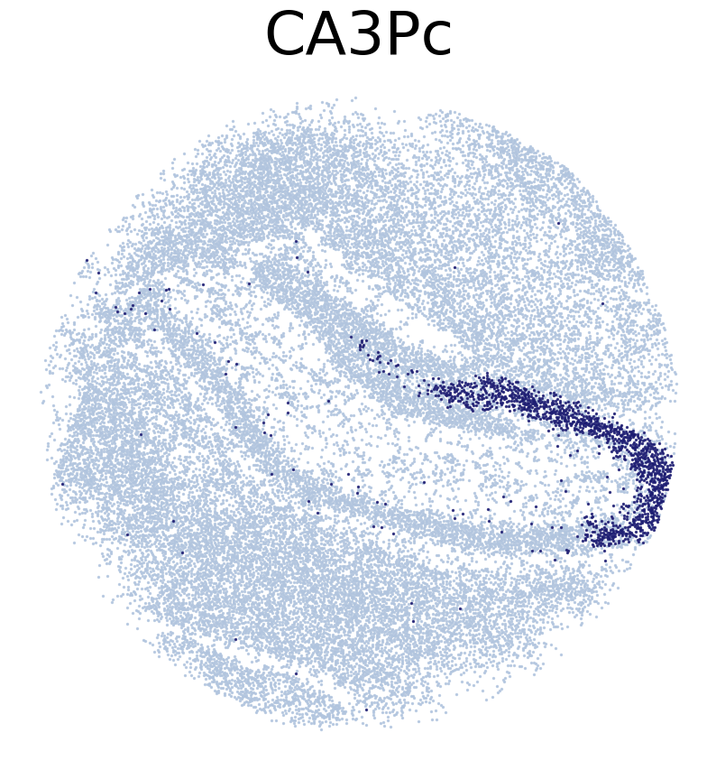
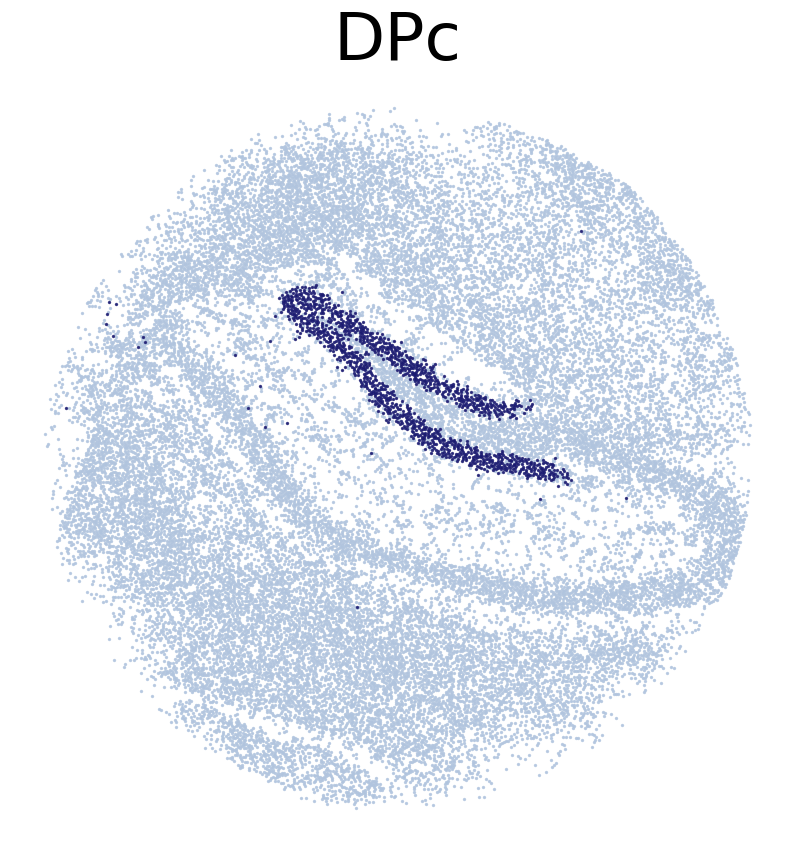
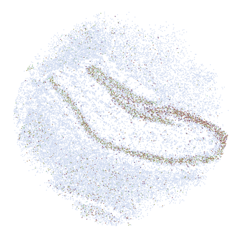
Draw reference ST data
[22]:
# True location of ST voxels. ST voxels were annotated by RCTD

CT_list = ['CA1Pc',
           'CA3Pc',
           'DPc']

#for CT in adata_ref.obs['celltype_1'].unique():
for CT in CT_list:
    print('*'*16)
    print(CT)
    print('*'*16)
    print('Transfer:')
    pl.DrawCT1(adata_ref, coords_name = 'spatial',
                CT = CT, FM = True, c_name = 'SSV2',
                root = 'tutorial1/Transfer2/FM_Valid2/', save = 'HC1')
****************
CA1Pc
****************
Transfer:

****************
CA3Pc
****************
Transfer:
****************
DPc
****************
Transfer:
Imputation
[28]:
#Draw a colorbar legend
from matplotlib import rc
import matplotlib.pyplot as plt
import seaborn as sns
import numpy as np
import pylab as pylabpl
rc('font', **{'family':'Arial','sans-serif':['Arial']})
plt.rcParams['font.size'] = 16

cmap = sns.cubehelix_palette(n_colors = 32,start = 2, rot=1.5, as_cmap = True)

a = np.array([[0,1]])
pylabpl.figure(figsize=(9, 1.5))
img = pylabpl.imshow(a, cmap=cmap)
pylabpl.gca().set_visible(False)
cax = pylabpl.axes([0, 0, 0.02, 1.6])
pylabpl.colorbar(orientation="vertical", cax=cax)
pylabpl.savefig("tutorial1/Transfer2/colorbar.png", bbox_inches='tight')
[30]:
#Pre-calculation for imputation
sta = time()

neighbors, dis = tl.NRD_CT_preprocess(adata_ref, adata_query,
                                      n_neighbors=1000, dis_cutoff=15)
tl.NRD_CT(neighbors, dis, adata_ref, adata_query,
          ct_name = 'simp_name', weight_constant=1, exclude_CTs = ['nan'])

end = time()
print((end - sta) / 60, 'min(s)')
0.6957667787869771 min(s)
[31]:
# Draw cell type proportion of ST voxels inferred based on SC2Spa's prediction
cmap = sns.cubehelix_palette(n_colors = 32,start = 2, rot=1.5, as_cmap = True)

CT_list = ['CA1 Principal cells',
           'CA2 Principal cells',
           'CA3 Principal cells',
           'Dentate Principal cells']

#for CT in adata_query.obs['simp_name'].unique():
for CT in CT_list:
    if(CT in ['nan']):
        continue
    print(CT)
    pl.DrawCT2(adata_ref, CT, title = True, coords_name = 'spatial', NRD = True, cmap=cmap, s=2,
               root='tutorial1/Transfer2/FM_NRD/', save='SC2HC1')
CA1 Principal cells
CA2 Principal cells

CA3 Principal cells
Dentate Principal cells
[32]:
# Impute gene expression of ST voxels
sta = time()

adata_impute = tl.NRD_impute(neighbors, dis, adata_ref, adata_query,
                             ct_name='simp_name', weight_constant=1, exclude_CTs=['nan'])

end = time()
print((end - sta) / 60, 'min(s)')
1.2381447752316792 min(s)
Ranking Genes by Their Contribution to Location Prediction
In this section, we aim to rank genes according to their contribution to predicting spatial locations in the dataset. This process is essential for identifying genes that exhibit significant spatial variability in their expression patterns.
- Identify Common Genes:We first identify the genes that are common between the reference (Slide-seqV2) and query (scRNA-seq) datasets. These genes form the basis for our analysis of spatial variability.
- Subset the Data:Using the identified common genes, we subset the reference dataset (
adata_ref). This step ensures that we focus only on genes relevant to both datasets, optimizing our analysis. - Train the Self-Mapping Model:Utilizing the subsetted reference dataset, we train a self-mapping model (
model). This model is designed to predict spatial locations based on gene expression patterns, incorporating sparse data handling for efficiency. - Prioritize Location-Predictive Genes:With the trained model, we prioritize genes based on their predictive power for spatial locations. Each gene is assigned an importance score (
imp_sumup_norm), which reflects its contribution to spatial prediction after normalization and scaling (scale_factor = 1e3). - Rank and Display Top Genes:Finally, we rank the genes in the reference dataset (
adata.var) according to theirimp_sumup_normscores in descending order. This ranking allows us to identify and focus on genes that play a significant role in predicting spatial locations, with higher scores indicating greater predictive importance.
By following these steps, we can systematically analyze and understand the spatial variability of gene expression within the dataset, highlighting genes that are crucial for spatial lcation prediction.
[33]:
# Rank genes according to their contribution to location prediction.
# The location predictive genes are spatial variable
JGs = sorted(list(set(adata_ref.var_names).intersection(set(adata_query.var_names))))
adata = adata_ref[:, JGs]

model = tl.Self_Mapping(adata, sparse = True, model_path = 'tutorial1/SI_T2.h5')

sva.PrioritizeLPG(adata, Model = model, percent = 0.5, scale_factor = 1e3,
                  Norm = True)

adata.var.sort_values('imp_sumup_norm', ascending = False).head()
<keras.layers.core.dense.Dense object at 0x7f42386d3e80> :
(4, 2)
<keras.layers.core.dense.Dense object at 0x7f423878bbe0> :
(16, 4)
<keras.layers.core.dense.Dense object at 0x7f423864e5f0> :
(64, 16)
<keras.layers.core.dense.Dense object at 0x7f42521ab430> :
(256, 64)
<keras.layers.core.dense.Dense object at 0x7f4252b350c0> :
(1024, 256)
<keras.layers.core.dense.Dense object at 0x7f423867f880> :
(4096, 1024)
<keras.layers.core.dense.Dense object at 0x7f4238630ac0> :
(19986, 4096)
[33]:
| n_cells | mt | ERCC | n_cells_by_counts | mean_counts | pct_dropout_by_counts | total_counts | imp_sumup | imp_sumup_norm | |
|---|---|---|---|---|---|---|---|---|---|
| TTR | 13069 | False | False | 13069 | 4.758839 | 67.090552 | 188983.0 | 1.477345 | 1.262538 |
| TSHZ2 | 2603 | False | False | 2603 | 0.105535 | 93.445306 | 4191.0 | 1.253887 | 1.071571 |
| PCP4 | 21317 | False | False | 21317 | 1.950670 | 46.321011 | 77465.0 | 1.197442 | 1.023334 |
| SST | 2943 | False | False | 2943 | 0.229452 | 92.589142 | 9112.0 | 1.075541 | 0.919156 |
| CALB2 | 3967 | False | False | 3967 | 0.193392 | 90.010576 | 7680.0 | 0.998086 | 0.852964 |
[34]:
cmap = sns.cubehelix_palette(n_colors = 32,start = 2, rot=1.5, as_cmap = True)

def VizCus(df, x_name, x_label, y_name, y_label, c_name = None,
           fontsize = 28, vmin= -0.05, vmax = 0.5, s = 14, save = None):

    plt.rcParams['font.size'] = fontsize
    plt.figure(figsize = (12, 8))
    if(c_name == None):
        plt.scatter(df[x_name], df[y_name], s = s)
    elif(vmin!=None):
        plt.scatter(df[x_name], df[y_name], s = s, alpha = 0.7,
                c = df[c_name], vmin = vmin, vmax = vmax, cmap = cmap)
    else:
        plt.scatter(df[x_name], df[y_name], s = s, alpha = 0.7,
                c = df[c_name], cmap = cmap)
    plt.colorbar()
    plt.xlabel(x_label)
    plt.ylabel(y_label)

    if(save != None):
        plt.savefig(save + '.png',
                    dpi = 128, bbox_inches='tight')
[ ]:
# This step is time consuming. Let's download precalculated stats file

'''
from scipy import stats
from IPython.display import clear_output

JCs = sorted(list(set(adata_ref.obs_names).intersection(set(adata_impute.obs_names))))

pearson_JGs = pd.DataFrame(np.zeros((len(JGs), 3)), columns = ['gene', 'pearson_r', 'p'])
pearson_JGs['gene'] = JGs

for i, JG in enumerate(JGs):
    print(i)
    t = stats.pearsonr(adata_impute[JCs, JG].X.flatten(), adata_ref[JCs, JG].X.toarray().flatten())
    pearson_JGs.loc[i, 'pearson_r'] = t[0]
    pearson_JGs.loc[i, 'p'] = t[1]
    clear_output(wait = True)
'''
[ ]:
'''
sc.pp.calculate_qc_metrics(adata, percent_top=None, log1p=False, inplace=True)
adata.var['percent_cell'] = adata.var['n_cells_by_counts'] / adata.shape[0]

t = adata.var[['percent_cell', 'imp_sumup_norm']].reset_index()
t.columns =['gene', 'percent_cell', 'imp_sumup_norm']
pearson_JGs = pearson_JGs.merge(t, how = 'left')

pearson_JGs.sort_values('pearson_r', ascending = False).to_csv('tutorial1/Transfer2/T2_stats.csv', index = None)
'''
[35]:
#Download precalculated stats file
!wget https://figshare.com/ndownloader/files/38940998 -O tutorial1/Transfer2/T2_stats.csv
pearson_JGs = pd.read_csv('tutorial1/Transfer2/T2_stats.csv')
pearson_JGs.sort_values('pearson_r', ascending = False).head(10)
--2023-07-31 18:46:29--  https://figshare.com/ndownloader/files/38940998
Resolving figshare.com (figshare.com)... 34.255.145.108, 34.240.187.105, 2a05:d018:1f4:d000:558e:605e:87f5:ced2, ...
Connecting to figshare.com (figshare.com)|34.255.145.108|:443... connected.
HTTP request sent, awaiting response... 302 Found
Location: https://s3-eu-west-1.amazonaws.com/pfigshare-u-files/38940998/T2_stats.csv?X-Amz-Algorithm=AWS4-HMAC-SHA256&X-Amz-Credential=AKIAIYCQYOYV5JSSROOA/20230731/eu-west-1/s3/aws4_request&X-Amz-Date=20230731T164630Z&X-Amz-Expires=10&X-Amz-SignedHeaders=host&X-Amz-Signature=485c0f8485bb303f6a9e271c20d602c1fd3ac0062340cf8d03401718d9550888 [following]
--2023-07-31 18:46:30--  https://s3-eu-west-1.amazonaws.com/pfigshare-u-files/38940998/T2_stats.csv?X-Amz-Algorithm=AWS4-HMAC-SHA256&X-Amz-Credential=AKIAIYCQYOYV5JSSROOA/20230731/eu-west-1/s3/aws4_request&X-Amz-Date=20230731T164630Z&X-Amz-Expires=10&X-Amz-SignedHeaders=host&X-Amz-Signature=485c0f8485bb303f6a9e271c20d602c1fd3ac0062340cf8d03401718d9550888
Resolving s3-eu-west-1.amazonaws.com (s3-eu-west-1.amazonaws.com)... 52.92.18.240, 52.218.40.147, 52.218.110.67, ...
Connecting to s3-eu-west-1.amazonaws.com (s3-eu-west-1.amazonaws.com)|52.92.18.240|:443... connected.
HTTP request sent, awaiting response... 200 OK
Length: 1615739 (1.5M) [text/csv]
Saving to: ‘tutorial1/Transfer2/T2_stats.csv’

tutorial1/Transfer2 100%[===================>]   1.54M  6.76MB/s    in 0.2s

2023-07-31 18:46:30 (6.76 MB/s) - ‘tutorial1/Transfer2/T2_stats.csv’ saved [1615739/1615739]
[35]:
| gene | pearson_r | p | percent_cell | imp_sumup_norm | |
|---|---|---|---|---|---|
| 0 | HPCA | 0.403153 | 0.000000e+00 | 0.417636 | 0.772095 |
| 1 | C1QL2 | 0.375441 | 0.000000e+00 | 0.031627 | 0.226433 |
| 2 | 6030445D17RIK | 0.360912 | 0.000000e+00 | 0.000283 | 0.002228 |
| 3 | NRGN | 0.321082 | 2.395553e-271 | 0.377210 | 0.755274 |
| 4 | FIBCD1 | 0.307258 | 1.685399e-247 | 0.033579 | 0.111303 |
| 5 | TSHZ2 | 0.302188 | 4.506501e-239 | 0.069252 | 1.071571 |
| 6 | PPP3CA | 0.298777 | 1.695301e-233 | 0.451837 | 0.485366 |
| 7 | CPNE6 | 0.289595 | 7.320895e-219 | 0.117457 | 0.326439 |
| 8 | OLFM1 | 0.277887 | 5.583135e-201 | 0.469150 | 0.482522 |
| 9 | HS3ST4 | 0.276645 | 3.930274e-199 | 0.091148 | 0.423905 |
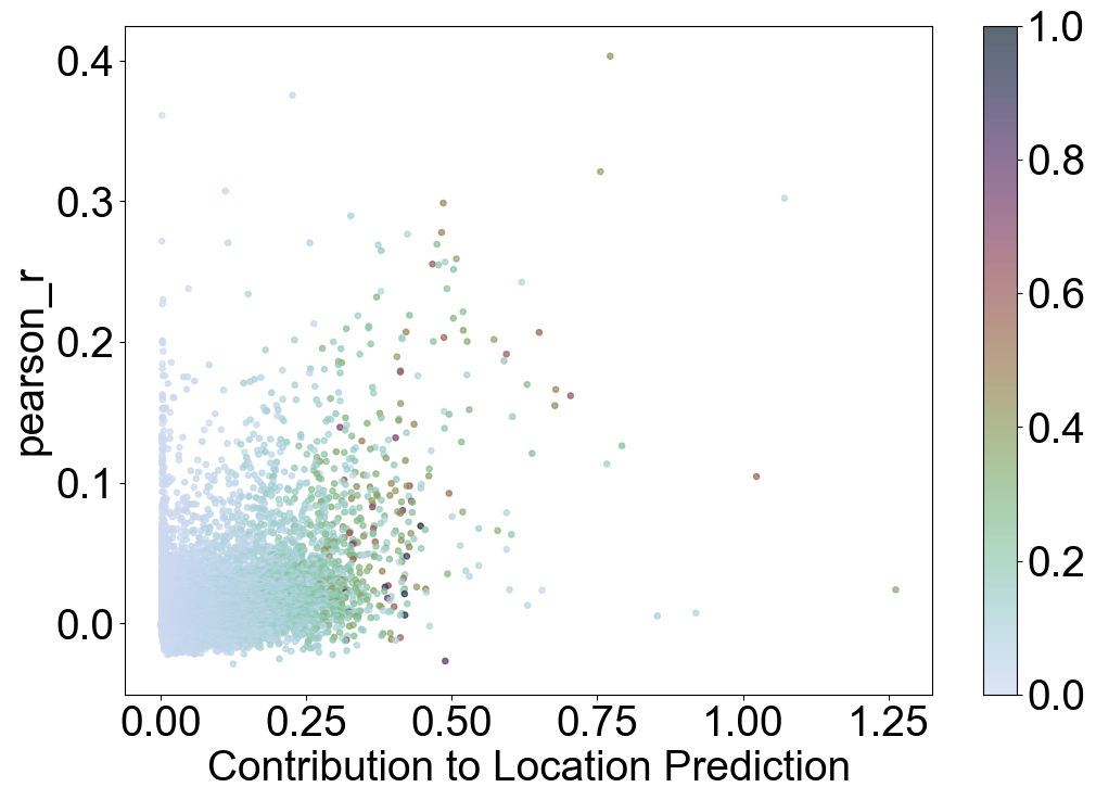
Visualizing Relationship Between Gene Importance and Pearson Correlation
This visualization explores how genes’ importance in predicting spatial locations (imp_sumup_norm) correlates with their Pearson correlation (pearson_r) and percentage of expression (percent_cell).
Key Points:
X-axis (``x_name``): Contribution to Location Prediction (
imp_sumup_norm)Genes with higher values on this axis contribute more to predicting spatial locations.
Y-axis (``y_name``): Pearson Correlation (
pearson_r)This measures the strength and direction of the linear relationship in gene expression across cells.
Point Size (``s``): 14
Each gene is represented by a marker with a fixed size.
Color (``c_name``): Percentage of Cells (
percent_cell)Points are colored based on how widely the gene is expressed across cells, ranging from low (0) to high (1).
Trends Observed:
Genes that play a crucial role in predicting spatial locations (imp_sumup_norm) tend to exhibit higher Pe between the reference and query dataarson correlations (pearson_r) and are often expressed in a higher percentage of cells (percent_cell). This suggests that genes contributing significantly to spatial prediction also show stronger and more widespread expression patterns across the dataset.
Insight:
Analyzing this visualization provides insights into how gene importance for spatial prediction relates to their expression characteristics. It helps in understanding which genes may drive spatial variability in gene expression and how their expressiobetween the reference and query datasets ells in the dataset. gene expression dynamics.
[36]:
VizCus(pearson_JGs, x_name = 'imp_sumup_norm', x_label = 'Contribution to Location Prediction',
       y_name = 'pearson_r', y_label = 'pearson_r', s = 14, c_name = 'percent_cell',
       vmin = 0, vmax = 1, save = 'tutorial1/Transfer2_imp_r_pcell.png')
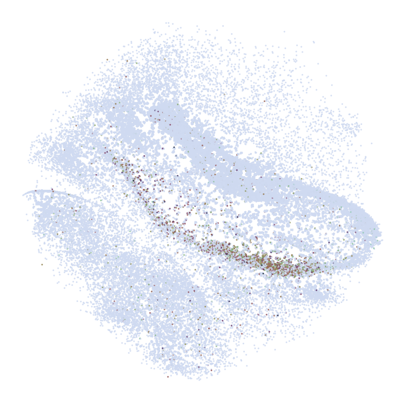
Visualizing Spatial Expression Patterns of Selected Genes
In e following cellon, we visualize the spatial expression patterns of selected genes (GLs) across different datasets: scRNA-seq (adata_query), Slide-seqV2 (adata_ref), and imputed Slide-seqV2 (adata_impute)fixed size.
Visualiza
Selected Genes (``GLs``): Top 10 Genes by Pearson Correlation
Genes with a significant Pearson correlation (
pearson_r) and expressed in more than 1% of cells are selected for visualization.
tion Details: For each selected gene (GLs), the following visualizations are generated:
scRNA-seq Data (``adata_query``):
Spatial expression pattern is visualized using
pl.DrawGenes2function with parameters tailored for scRNA-seq data.Coordinates are mapped using ‘spatial_mapping’ and cell type information is represented by color (‘simp_name’).
Slide-seqV2 Data (``adata_ref``):
Spatial expression pattern is visualized using
pl.DrawGenes2function with parameters specific to Slide-seqV2 data.Coordinates are mapped using ‘spatial’ and bead information is represented by color (‘SSV2’).
Imputed Slide-seqV2 Data (``adata_impute``):
Similar visualization as Slide-seqV2 data but for imputed gene expression patterns.referenceelps in comparing original vs. imputed spatial expression patterns for the selected genes.
Output:
Each visualization is saved in the directory ‘tutorial1/Transfer2/FM_Valid1/’ with filenames indicating the dataset and gene name (These visualizations compare spatial patterns of gene expression across the reference dataset, the query dataset, and the predicted results generated by the SC2Spa model.ial gene expression dynamics.
[37]:
cmap = sns.cubehelix_palette(n_colors = 32,start = 2, rot=1.5, as_cmap = True)

GLs = pearson_JGs[pearson_JGs['percent_cell']>0.01].sort_values('pearson_r', ascending = False)['gene'][:10]

GLs = list(set(GLs))
s = 4

for gene in GLs:
    print('*'*32)
    print(gene)
    print('*'*32)
    print('scRNAseq:')
    pl.DrawGenes2(adata_query, gene = gene, lim = False, coords_name = 'spatial_mapping',
                   xlim = [650, 5750], ylim = [650, 5750], cmap = cmap,
                   FM = True, CTL = None, c_name = 'simp_name',
                   root = 'tutorial1/Transfer2/FM_Valid1/', title = False, save = 'AMB')
    print('ST:')
    pl.DrawGenes2(adata_ref, gene = gene, lim = True,coords_name = 'spatial',
                   xlim = [650, 5750], ylim = [650, 5750], cmap = cmap,
                   FM = True, CTL = None, c_name = 'SSV2',
                   root = 'tutorial1/Transfer2/FM_Valid1/', title = False, save = 'HC1')
    print('Imputed ST:')
    pl.DrawGenes2(adata_impute, gene = gene, lim = True, coords_name = 'spatial',
                   xlim = [650, 5750], ylim = [650, 5750], cmap = cmap,
                   FM = True, CTL = None, c_name = 'SSV2',
                   root = 'tutorial1/Transfer2/FM_Valid1/', title = False, save = 'HC1_Impute')
********************************
FIBCD1
********************************
scRNAseq:
ST:

Imputed ST:
********************************
NRGN
********************************
scRNAseq:
ST:

Imputed ST:
********************************
C1QL2
********************************
scRNAseq:
ST:

Imputed ST:
********************************
PPP3CA
********************************
scRNAseq:
ST:
Imputed ST:
********************************
OLFM1
********************************
scRNAseq:
ST:

Imputed ST:
********************************
TSHZ2
********************************
scRNAseq:

ST:
Imputed ST:

********************************
HPCA
********************************
scRNAseq:

ST:

Imputed ST:
********************************
PROX1
********************************
scRNAseq:
ST:
Imputed ST:
********************************
HS3ST4
********************************
scRNAseq:
ST:

Imputed ST:
********************************
CPNE6
********************************
scRNAseq:
ST:
Imputed ST: