Map snRNAseq to Visium (Cell2Location Adult Mouse Brain)
[1]:
import os
from time import time

import anndata as ad
import scanpy as sc
from SC2Spa import tl, pp, pl, sva

import pandas as pd

from numpy.random import seed
from tensorflow.random import set_seed
import tensorflow as tf
2024-07-07 19:24:42.126954: I tensorflow/core/util/port.cc:113] oneDNN custom operations are on. You may see slightly different numerical results due to floating-point round-off errors from different computation orders. To turn them off, set the environment variable `TF_ENABLE_ONEDNN_OPTS=0`.
2024-07-07 19:24:42.168881: E external/local_xla/xla/stream_executor/cuda/cuda_dnn.cc:9261] Unable to register cuDNN factory: Attempting to register factory for plugin cuDNN when one has already been registered
2024-07-07 19:24:42.168907: E external/local_xla/xla/stream_executor/cuda/cuda_fft.cc:607] Unable to register cuFFT factory: Attempting to register factory for plugin cuFFT when one has already been registered
2024-07-07 19:24:42.170105: E external/local_xla/xla/stream_executor/cuda/cuda_blas.cc:1515] Unable to register cuBLAS factory: Attempting to register factory for plugin cuBLAS when one has already been registered
2024-07-07 19:24:42.176544: I tensorflow/core/platform/cpu_feature_guard.cc:182] This TensorFlow binary is optimized to use available CPU instructions in performance-critical operations.
To enable the following instructions: AVX2 AVX512F AVX512_VNNI FMA, in other operations, rebuild TensorFlow with the appropriate compiler flags.
2024-07-07 19:24:44.861742: W tensorflow/compiler/tf2tensorrt/utils/py_utils.cc:38] TF-TRT Warning: Could not find TensorRT
[2]:
import SC2Spa

print(SC2Spa.__all__)
print('*'*20)
print('Version:', SC2Spa.__version__)
['__title__', '__summary__', '__uri__', '__version__', '__author__', '__email__', '__license__', '__copyright__']
********************
Version: 1.3.0
Download processed datasets and pretrained model
Datasets
Cell2Location_ST.h5ad
Spatial reference data
Visium mouse brain data from the Cell2Location paper
Downloaded to:
Dataset/Cell2Location_ST.h5ad
Cell2Location_snRNAseq.h5ad
snRNAseq query data
Mouse brain data from Cell2Location paper
Downloaded to:
Dataset/Cell2Location_snRNAseq.h5ad
WDs_snRNAseq2Visium.csv
Gene Wasserstein distances between the reference and query data
Used to select genes with similar distribution between reference and query
These selected genes are used for training the SC2Spa model
Downloaded to:
Dataset/WDs_snRNAseq2Visium.csv
Pretrained Model
Cell2Location_snRNAseq2ST_SC2Spa_WD.h5
Pretrained SC2Spa model
Used for mapping the snRNAseq data to the spatial reference data
Downloaded to:
Model/Cell2Location_snRNAseq2ST_SC2Spa_WD.h5
Download Process
Create a ‘Dataset’ directory if it doesn’t exist
Download the spatial reference data (Cell2Location_ST.h5ad)
Download the snRNAseq query data (Cell2Location_snRNAseq.h5ad)
Download the Gene Wasserstein distances file (WDs_snRNAseq2Visium.csv)
Create a ‘Model’ directory if it doesn’t exist
Download the pretrained SC2Spa model (Cell2Location_snRNAseq2ST_SC2Spa_WD.h5)
This process ensures all necessary files are downloaded and organized in the appropriate directories for subsequent analysis.
[23]:
if not os.path.exists('Dataset'):
    os.makedirs('Dataset')
!wget https://figshare.com/ndownloader/files/47474501 -O Dataset/Cell2Location_ST.h5ad
!wget https://figshare.com/ndownloader/files/47474504 -O Dataset/Cell2Location_snRNAseq.h5ad

if not os.path.exists('Model'):
    os.makedirs('Model')
!wget https://figshare.com/ndownloader/files/47485421 -O Model/Cell2Location_snRNAseq2ST_SC2Spa_WD.h5
--2024-07-07 23:22:19-- https://figshare.com/ndownloader/files/47474501
/home/liaol/anaconda3/lib/python3.11/pty.py:89: RuntimeWarning: os.fork() was called. os.fork() is incompatible with multithreaded code, and JAX is multithreaded, so this will likely lead to a deadlock.
  pid, fd = os.forkpty()
Resolving figshare.com (figshare.com)... 34.251.213.12, 52.31.138.59, 2a05:d018:1f4:d003:5aa0:a091:6220:4fef, ...
Connecting to figshare.com (figshare.com)|34.251.213.12|:443... connected.
HTTP request sent, awaiting response... 302 Found
Location: https://s3-eu-west-1.amazonaws.com/pfigshare-u-files/47474501/Cell2Location_ST.h5ad?X-Amz-Algorithm=AWS4-HMAC-SHA256&X-Amz-Credential=AKIAIYCQYOYV5JSSROOA/20240708/eu-west-1/s3/aws4_request&X-Amz-Date=20240708T062220Z&X-Amz-Expires=10&X-Amz-SignedHeaders=host&X-Amz-Signature=7bda0b75f779b1372a91392df49df75a1d3ff41006fdb34fc8bd07e62ae36756 [following]
--2024-07-07 23:22:20--  https://s3-eu-west-1.amazonaws.com/pfigshare-u-files/47474501/Cell2Location_ST.h5ad?X-Amz-Algorithm=AWS4-HMAC-SHA256&X-Amz-Credential=AKIAIYCQYOYV5JSSROOA/20240708/eu-west-1/s3/aws4_request&X-Amz-Date=20240708T062220Z&X-Amz-Expires=10&X-Amz-SignedHeaders=host&X-Amz-Signature=7bda0b75f779b1372a91392df49df75a1d3ff41006fdb34fc8bd07e62ae36756
Resolving s3-eu-west-1.amazonaws.com (s3-eu-west-1.amazonaws.com)... 52.218.25.195, 52.218.41.27, 52.218.89.3, ...
Connecting to s3-eu-west-1.amazonaws.com (s3-eu-west-1.amazonaws.com)|52.218.25.195|:443... connected.
HTTP request sent, awaiting response... 200 OK
Length: 41988844 (40M) [application/octet-stream]
Saving to: ‘Dataset/Cell2Location_ST.h5ad’

Dataset/Cell2Locati 100%[===================>]  40.04M  14.1MB/s    in 2.8s

2024-07-07 23:22:24 (14.1 MB/s) - ‘Dataset/Cell2Location_ST.h5ad’ saved [41988844/41988844]

--2024-07-07 23:22:25--  https://figshare.com/ndownloader/files/47474504
Resolving figshare.com (figshare.com)... 52.31.138.59, 34.251.213.12, 2a05:d018:1f4:d003:5aa0:a091:6220:4fef, ...
Connecting to figshare.com (figshare.com)|52.31.138.59|:443... connected.
HTTP request sent, awaiting response... 302 Found
Location: https://s3-eu-west-1.amazonaws.com/pfigshare-u-files/47474504/Cell2Location_snRNAseq.h5ad?X-Amz-Algorithm=AWS4-HMAC-SHA256&X-Amz-Credential=AKIAIYCQYOYV5JSSROOA/20240708/eu-west-1/s3/aws4_request&X-Amz-Date=20240708T062226Z&X-Amz-Expires=10&X-Amz-SignedHeaders=host&X-Amz-Signature=80b47b0d4b4a4962f59a9e224257dac94b858a1fa65561b2ef90dfef5df7da4f [following]
--2024-07-07 23:22:26--  https://s3-eu-west-1.amazonaws.com/pfigshare-u-files/47474504/Cell2Location_snRNAseq.h5ad?X-Amz-Algorithm=AWS4-HMAC-SHA256&X-Amz-Credential=AKIAIYCQYOYV5JSSROOA/20240708/eu-west-1/s3/aws4_request&X-Amz-Date=20240708T062226Z&X-Amz-Expires=10&X-Amz-SignedHeaders=host&X-Amz-Signature=80b47b0d4b4a4962f59a9e224257dac94b858a1fa65561b2ef90dfef5df7da4f
Resolving s3-eu-west-1.amazonaws.com (s3-eu-west-1.amazonaws.com)... 52.218.0.83, 52.92.33.0, 52.218.63.43, ...
Connecting to s3-eu-west-1.amazonaws.com (s3-eu-west-1.amazonaws.com)|52.218.0.83|:443... connected.
HTTP request sent, awaiting response... 200 OK
Length: 235097048 (224M) [application/octet-stream]
Saving to: ‘Dataset/Cell2Location_snRNAseq.h5ad’

Dataset/Cell2Locati 100%[===================>] 224.21M  19.8MB/s    in 27s

2024-07-07 23:22:54 (8.31 MB/s) - ‘Dataset/Cell2Location_snRNAseq.h5ad’ saved [235097048/235097048]

--2024-07-07 23:22:55--  https://figshare.com/ndownloader/files/47485421
Resolving figshare.com (figshare.com)... 52.31.138.59, 34.251.213.12, 2a05:d018:1f4:d000:4856:ab6:5d9e:fe0e, ...
Connecting to figshare.com (figshare.com)|52.31.138.59|:443... connected.
HTTP request sent, awaiting response... 302 Found
Location: https://s3-eu-west-1.amazonaws.com/pfigshare-u-files/47485421/ModelCell2Location_snRNAseq2ST_SC2Spa_WD.h5?X-Amz-Algorithm=AWS4-HMAC-SHA256&X-Amz-Credential=AKIAIYCQYOYV5JSSROOA/20240708/eu-west-1/s3/aws4_request&X-Amz-Date=20240708T062256Z&X-Amz-Expires=10&X-Amz-SignedHeaders=host&X-Amz-Signature=ac474350f6ab127d4d1158b89d03ccdb315eb29ba3f6973a3aa260be0ef6e4ce [following]
--2024-07-07 23:22:56--  https://s3-eu-west-1.amazonaws.com/pfigshare-u-files/47485421/ModelCell2Location_snRNAseq2ST_SC2Spa_WD.h5?X-Amz-Algorithm=AWS4-HMAC-SHA256&X-Amz-Credential=AKIAIYCQYOYV5JSSROOA/20240708/eu-west-1/s3/aws4_request&X-Amz-Date=20240708T062256Z&X-Amz-Expires=10&X-Amz-SignedHeaders=host&X-Amz-Signature=ac474350f6ab127d4d1158b89d03ccdb315eb29ba3f6973a3aa260be0ef6e4ce
Resolving s3-eu-west-1.amazonaws.com (s3-eu-west-1.amazonaws.com)... 52.218.122.96, 52.92.16.160, 52.218.118.80, ...
Connecting to s3-eu-west-1.amazonaws.com (s3-eu-west-1.amazonaws.com)|52.218.122.96|:443... connected.
HTTP request sent, awaiting response... 200 OK
Length: 573692024 (547M) [application/octet-stream]
Saving to: ‘Model/Cell2Location_snRNAseq2ST_SC2Spa_WD.h5’

Model/Cell2Location 100%[===================>] 547.12M  19.3MB/s    in 29s

2024-07-07 23:23:26 (18.8 MB/s) - ‘Model/Cell2Location_snRNAseq2ST_SC2Spa_WD.h5’ saved [573692024/573692024]
[4]:
!wget https://figshare.com/ndownloader/files/47484764 -O Dataset/WDs_snRNAseq2Visium.csv
--2024-07-07 21:49:58--  https://figshare.com/ndownloader/files/47484764
Resolving figshare.com (figshare.com)... 108.128.102.72, 54.155.22.15, 2a05:d018:1f4:d000:7204:fe27:5e76:7502, ...
Connecting to figshare.com (figshare.com)|108.128.102.72|:443... connected.
HTTP request sent, awaiting response... 302 Found
Location: https://s3-eu-west-1.amazonaws.com/pfigshare-u-files/47484764/WDs_snRNAseq2Visium.csv?X-Amz-Algorithm=AWS4-HMAC-SHA256&X-Amz-Credential=AKIAIYCQYOYV5JSSROOA/20240708/eu-west-1/s3/aws4_request&X-Amz-Date=20240708T044959Z&X-Amz-Expires=10&X-Amz-SignedHeaders=host&X-Amz-Signature=60779cde6c198975d2d4db6e5d59afb5db21bd6235338a8aa3a8f7abc6bec6fa [following]
--2024-07-07 21:49:59--  https://s3-eu-west-1.amazonaws.com/pfigshare-u-files/47484764/WDs_snRNAseq2Visium.csv?X-Amz-Algorithm=AWS4-HMAC-SHA256&X-Amz-Credential=AKIAIYCQYOYV5JSSROOA/20240708/eu-west-1/s3/aws4_request&X-Amz-Date=20240708T044959Z&X-Amz-Expires=10&X-Amz-SignedHeaders=host&X-Amz-Signature=60779cde6c198975d2d4db6e5d59afb5db21bd6235338a8aa3a8f7abc6bec6fa
Resolving s3-eu-west-1.amazonaws.com (s3-eu-west-1.amazonaws.com)... 52.92.16.120, 52.218.1.19, 52.218.24.179, ...
Connecting to s3-eu-west-1.amazonaws.com (s3-eu-west-1.amazonaws.com)|52.92.16.120|:443... connected.
HTTP request sent, awaiting response... 200 OK
Length: 523895 (512K) [text/csv]
Saving to: ‘Dataset/WDs_snRNAseq2Visium.csv’

Dataset/WDs_snRNAse 100%[===================>] 511.62K   876KB/s    in 0.6s

2024-07-07 21:50:01 (876 KB/s) - ‘Dataset/WDs_snRNAseq2Visium.csv’ saved [523895/523895]
Load
[15]:
#Load reference and query data
adata_ref = ad.read_h5ad('Dataset/Cell2Location_ST.h5ad')
adata_query = ad.read_h5ad('Dataset/Cell2Location_snRNAseq.h5ad')
[17]:
len(set(adata_ref.var_names).intersection(adata_query.var_names))
[17]:
19286
Select genes based on Wasserstein distance
This step filters genes based on their Wasserstein distance to identify those with similar distributions between the reference and query datasets.
Set the Wasserstein distance cutoff: ```python WD_cutoff = 0.1
[10]:
#Select genes with Warsserstein distance greater than 0.1
WD_cutoff = 0.1
WDs = pd.read_csv('Dataset/WDs_snRNAseq2Visium.csv')

JGs = sorted(WDs[WDs['Wasserstein_Distance'] < WD_cutoff]['Gene'].tolist())
[18]:
#10572 genes were selected
print(len(JGs))
10572
Set random seed and filter datasets
This step sets a consistent random seed for reproducibility and filters the reference and query datasets to include only the selected genes.
[21]:
## Set random seed
seed_num = 2022

seed(seed_num)
set_seed(seed_num)
tf.keras.utils.set_random_seed(seed_num)

adata_ref = adata_ref[:, JGs]
adata_query = adata_query[:, JGs]
Fine Mapping with SC2Spa
This section performs fine mapping of the query data onto the reference data using the SC2Spa model.
Starts a timer to measure the execution time of the FineMapping process
Calls the
FineMappingfunction from thetl(tools) modulePasses the reference (
adata_ref) and query (adata_query) data to the functionSets various parameters for the FineMapping process:
sparse = True: Indicates that sparse matrices should be usedmodel_path: Specifies the path to a pre-trained modelWD_cutoff,root, andnameare set toNone, using default valuesdis_cutoff = 110: Sets a distance cutoff for neighbor calculationsseed: Uses a predefined seed number for reproducibility
Ends the timer and prints the execution time in minutes
Key points:
The function used a pre-trained model for the mapping process
The process maps single-cell RNA-seq data to spatial transcriptomics data
The predicted spatial coordinates of the query data is stored in adata_query.obsm['spatial_mapping']
Note: For detailed usage information about the FineMapping function, you can use help(tl.FineMapping) in your Python environment.
[24]:
sta = time()

# Perform FineMapping analysis
tl.FineMapping(adata_ref, adata_query, sparse =True,
               model_path = 'Model/Cell2Location_snRNAseq2ST_SC2Spa_WD.h5',
               WD_cutoff = None, root = None, name = None,
               #l1_reg = 1e-5, l2_reg = 0, dropout = 0.05, epoch = 500, batch_size = 128,
               #nodes = [4096, 1024, 256, 64, 16, 4], lrr_patience = 20, ES_patience = 50,
               #min_lr = 1e-5, save = True, polar = True, n_neighbors = 1000,
               dis_cutoff = 110, seed = seed_num)

end = time()
print((end - sta) / 60.0, 'min')
n of Referece Genes: 10572
n of Target Genes: 10572
n of Selected Genes: 10572
(2983, 10572)
(40532, 10572)
1267/1267 [==============================] - 12s 9ms/step
94/94 [==============================] - 1s 9ms/step
0.3834413925806681 min
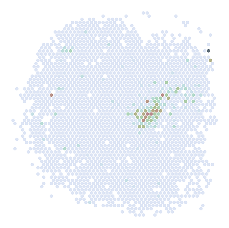
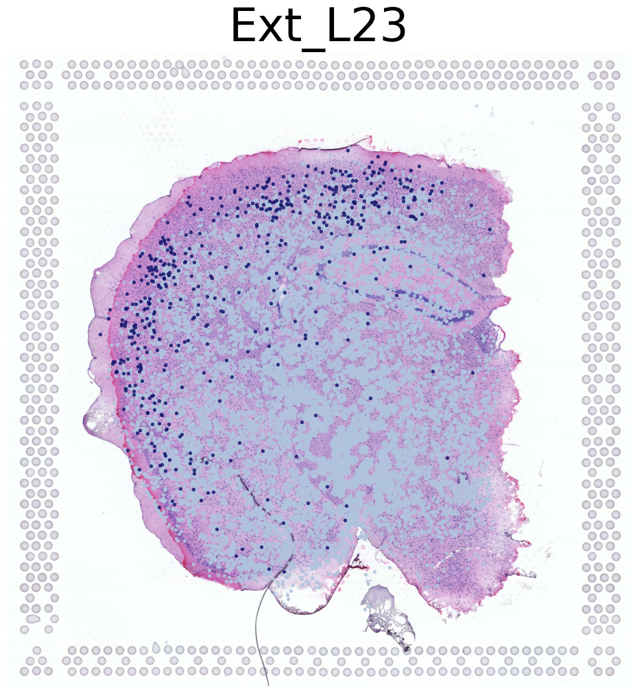
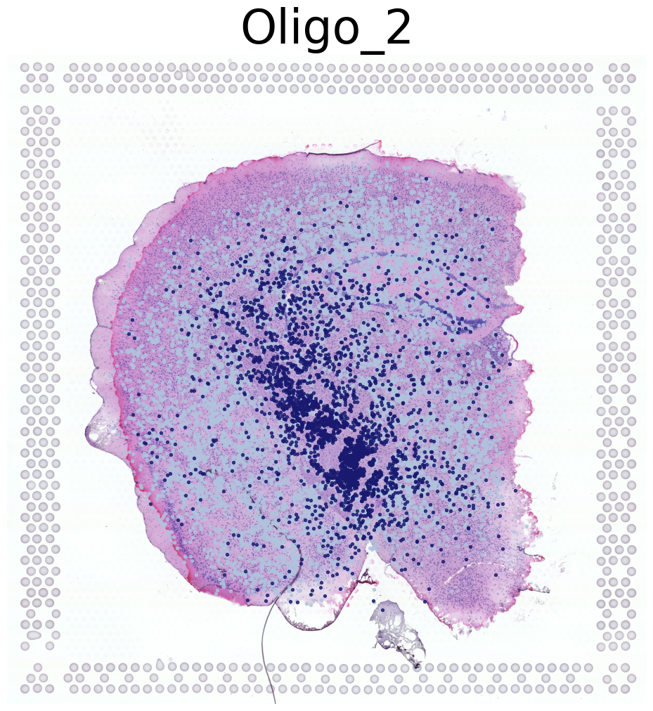
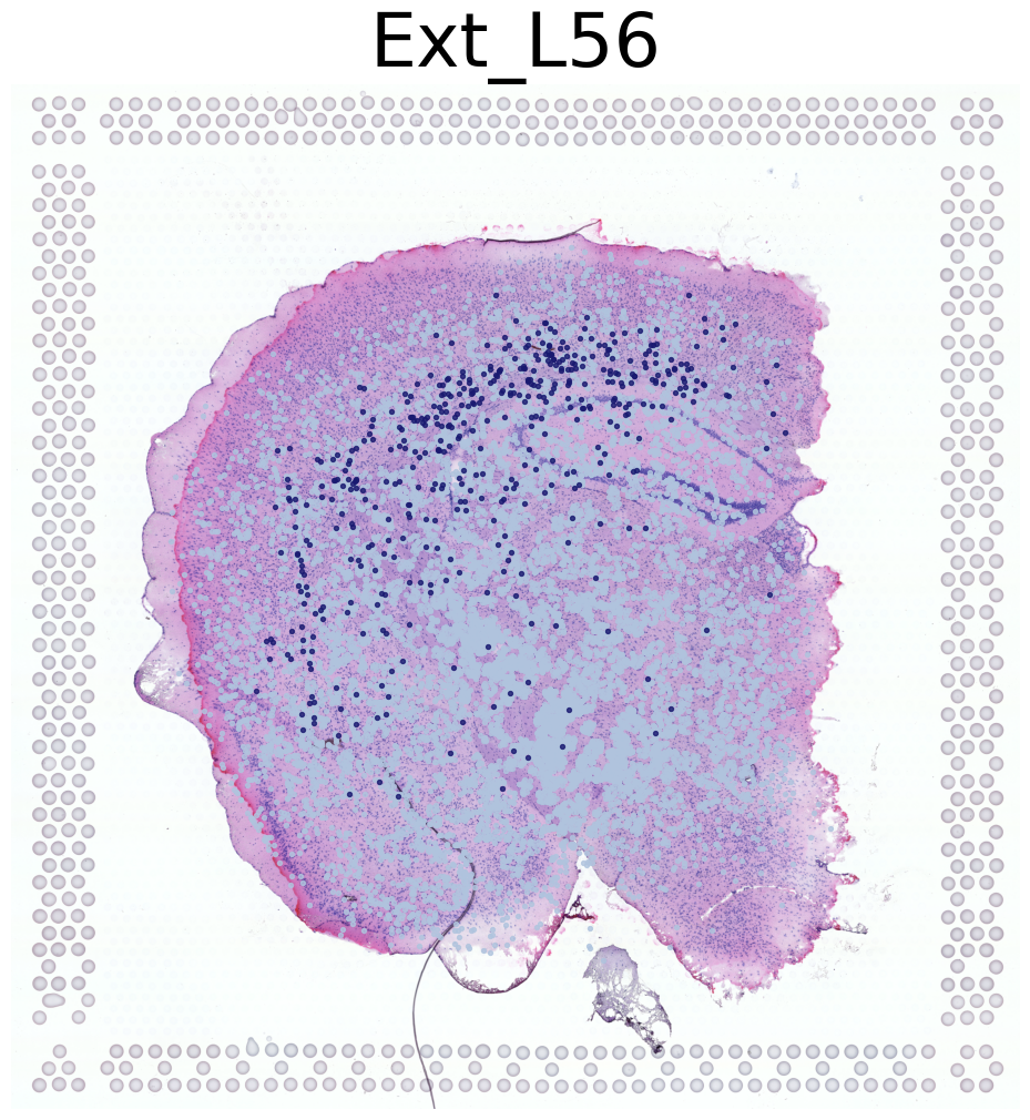
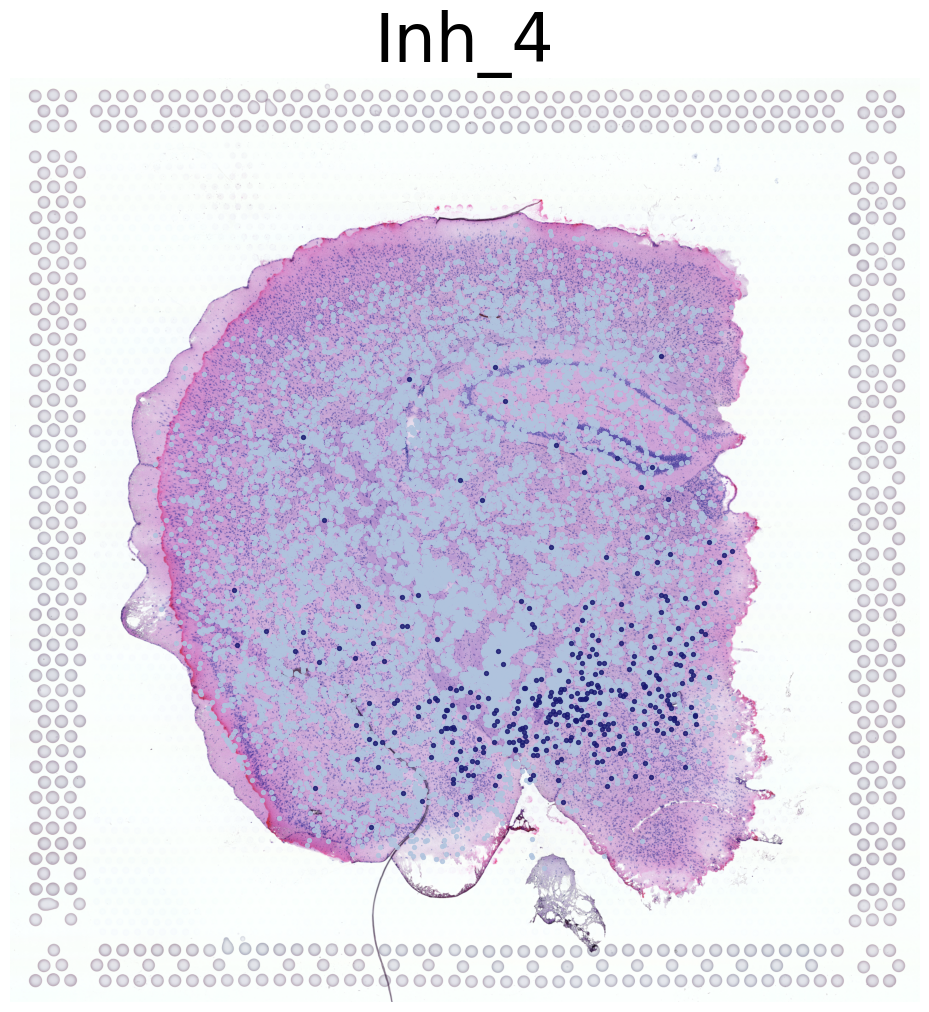
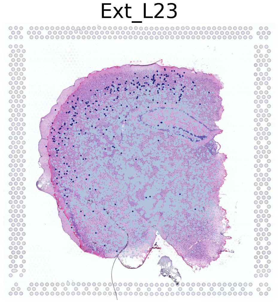
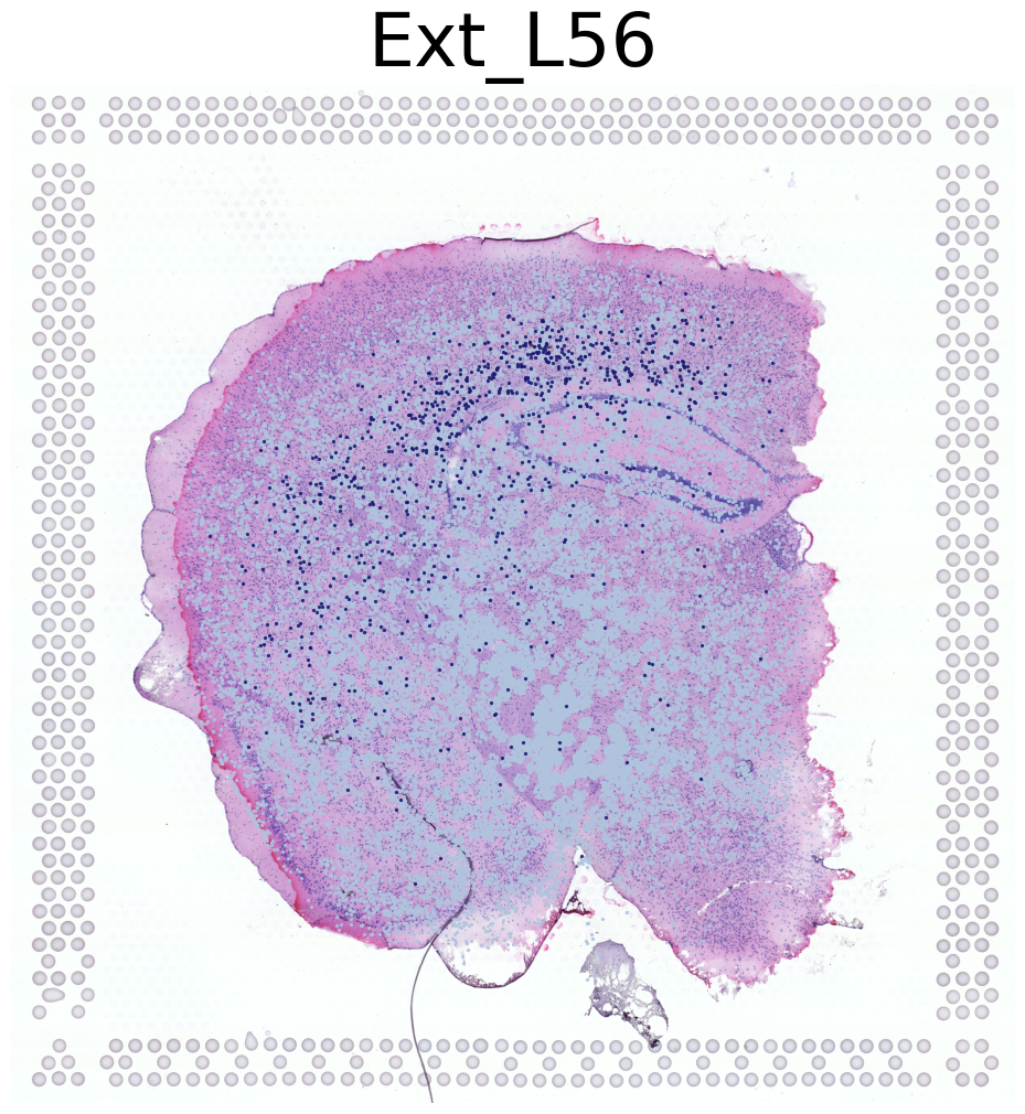
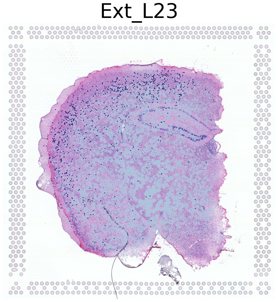
Visualize Cell Type Locations
This code visualizes the predicted locations of different cell types by SC2Spa.
This code:
Sets up the scale factor for high resolution visualization
Select specific individual samples (for mouse 1)
Iterates through cell types, visualizing up to 4 different types
For each cell type, it creates a figure showing the predicted locations overlaid on a high-resolution tissue image
Saves each visualization with a unique identifier
[26]:
import matplotlib.pyplot as plt

# Get the library ID and scale factor
lib_id = list(adata_ref.uns['spatial'].keys())[0]
scalef = adata_ref.uns['spatial'][lib_id]['scalefactors']['tissue_hires_scalef']
adata_query.obsm['spatial_mapping_hires'] =adata_query.obsm['spatial_mapping'] * scalef
# Define individual samples
individual1 = adata_query.obs['sample'].apply(lambda x: x in ['5705STDY8058280',
                                                             '5705STDY8058281',
                                                             '5705STDY8058282']).tolist()

# Visualize cell types
i = 0
for CT in adata_query.obs['annotation_1'].value_counts().index.tolist():
    print('*'*16)
    print(CT)
    print('*'*16)
    print('Transfer:')
    plt.figure(figsize = (12, 12))

    plt.imshow(adata_ref.uns['spatial'][lib_id]['images']['hires'])
    pl.DrawCT1(adata_query[individual1], coords_name='spatial_mapping_hires', CT = CT, s = 8, FM = True,
                c_name = 'annotation_1', root = 'Transfer' + str(i+1) +'/FM_Valid1/',
                figsize = None, save = 'T' + str(i+1) + '_individual1')
    i+=1
    if(i>3):
        break
****************
Oligo_2
****************
Transfer:
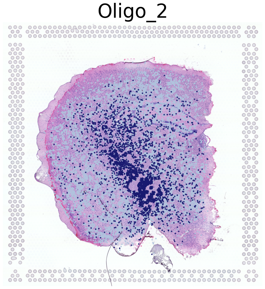
****************
Ext_L56
****************
Transfer:
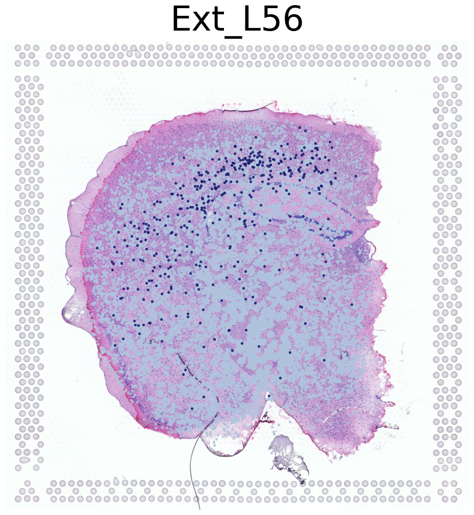
****************
Inh_4
****************
Transfer:
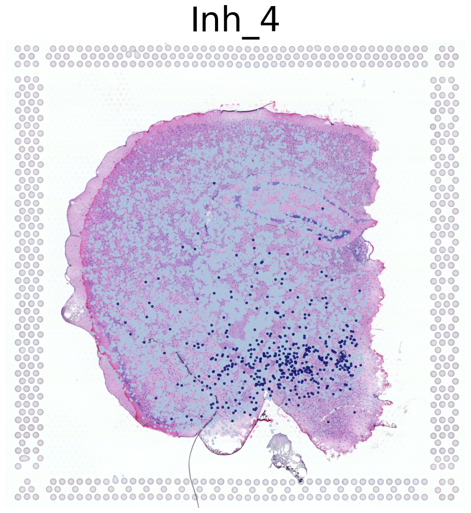
****************
Ext_L23
****************
Transfer:
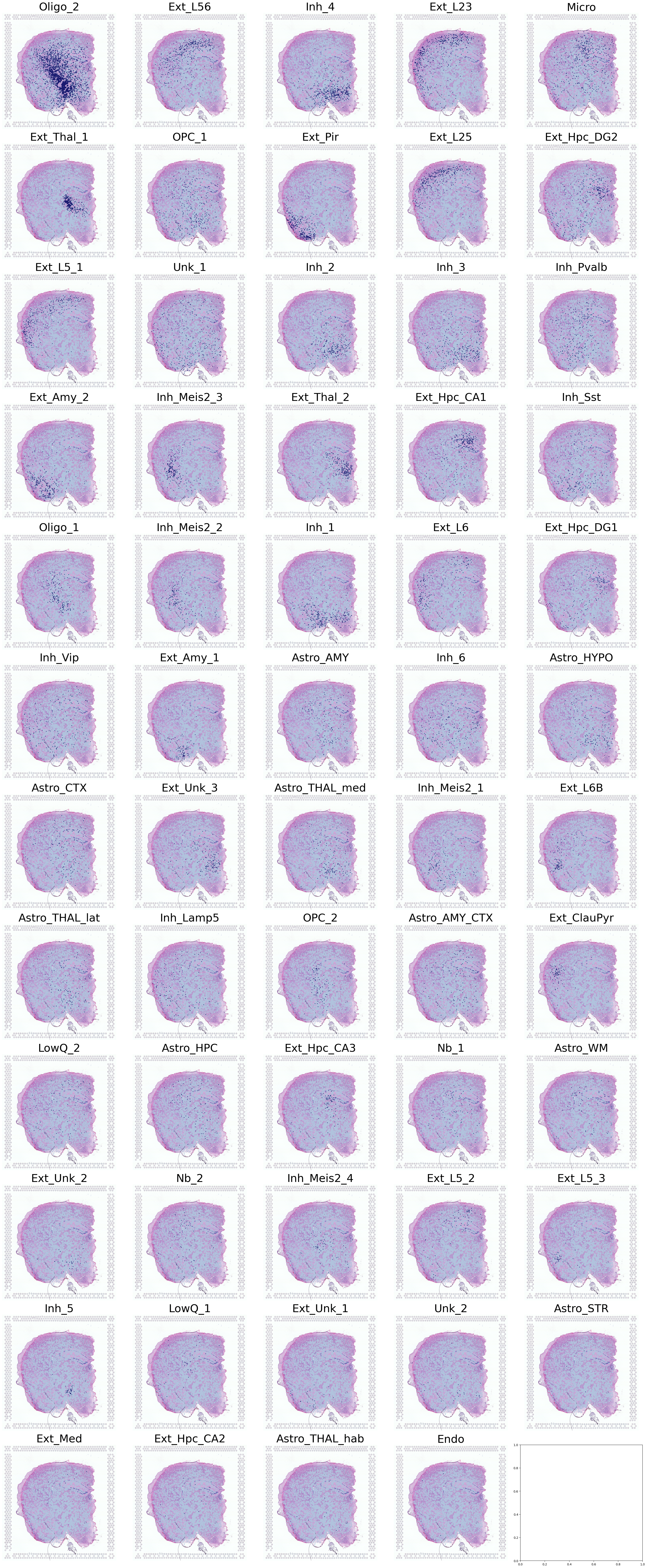
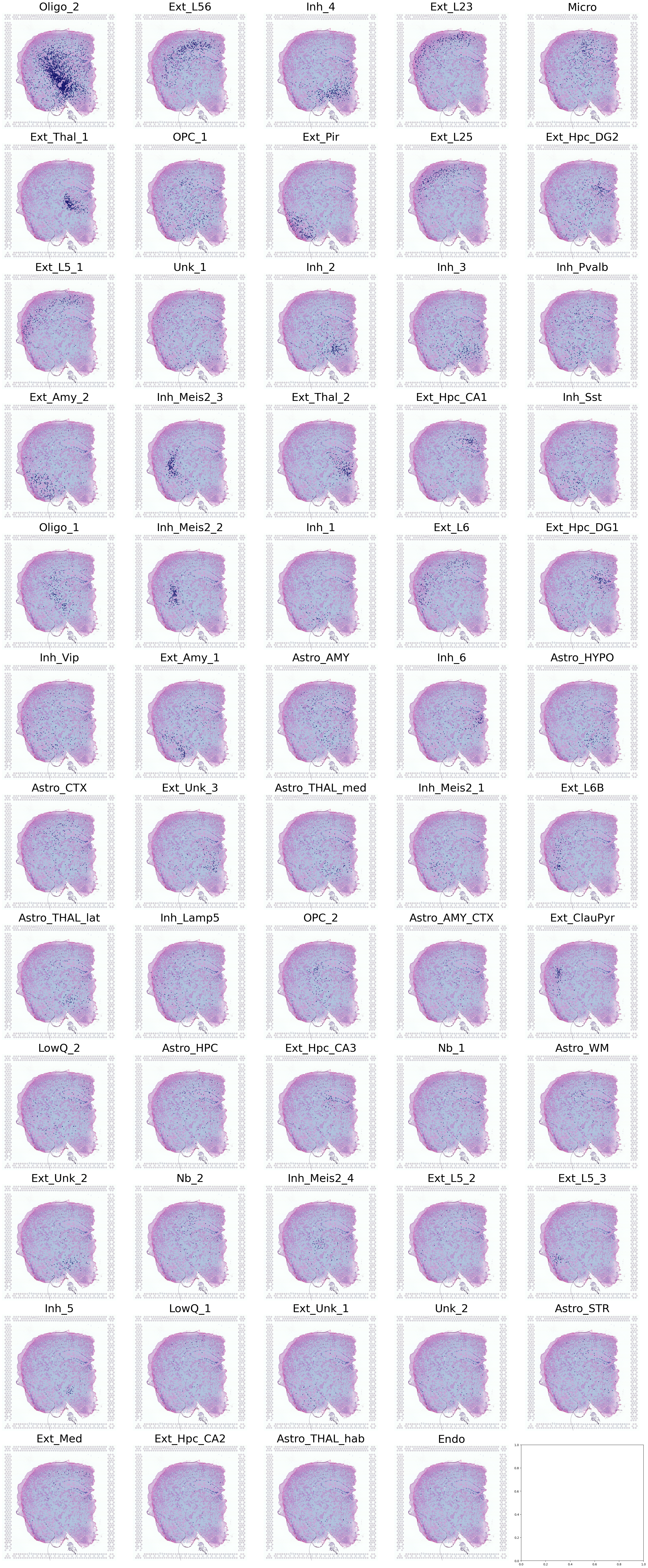
Visualization of Cell Types in Spatial Transcriptomics
This code creates a comprehensive visualization of multiple cell types in a spatial transcriptomics dataset.
Setup
Define grid parameters:
12 rows and 5 columns for a total of 60 subplots
Initialize variables:
Set up file paths for saving the output
Create a large figure with subplots
Prepare spatial data:
Extract the scale factor from the reference data
Apply the scale factor to create high-resolution spatial visualization
Select specific samples:
Filter for samples with IDs ‘5705STDY8058280’, ‘5705STDY8058281’, ‘5705STDY8058282’
These samples are from mouse/individual 1
Visualization Process
Iterate through cell types:
Use ‘annotation_1’ from the query data to get cell types
For each cell type:
Calculate its position in the subplot grid
Display the high-resolution tissue image as background
Overlay cell type locations using the
DrawCT1functionUse high-resolution spatial mapping
Set point size and color based on cell type
Adjust layout and save:
Apply tight layout to optimize subplot arrangement
Save the entire figure as a high-resolution PNG file
Output
A single large image containing up to 60 subplots
Each subplot represents a different cell type
Cell type locations are visualized on top of the tissue image
Saved as a high-resolution PNG file for further analysis
This visualization provides a comprehensive overview of the spatial distribution of multiple cell types within the tissue, allowing for easy comparison and analysis of cell type localization patterns.
[27]:
n_row = 12
n_col = 5
i = 0
root = 'Transfer' + str(i+1) +'/FM_Valid1/'
save = 'T' + str(i+1) + '_individual1'

fig, axes = plt.subplots(n_row, n_col, figsize = (6*n_col, 6*n_row))

lib_id = list(adata_ref.uns['spatial'].keys())[0]
scalef = adata_ref.uns['spatial'][lib_id]['scalefactors']['tissue_hires_scalef']
adata_query.obsm['spatial_mapping_hires'] =adata_query.obsm['spatial_mapping'] * scalef
individual1 = adata_query.obs['sample'].apply(lambda x: x in ['5705STDY8058280',
                                                              '5705STDY8058281',
                                                              '5705STDY8058282']).tolist()

for i, CT in enumerate(adata_query.obs['annotation_1'].value_counts().index.tolist()):

    i_row = int(i/n_col)
    i_col = int(i%n_col)

    axes[i_row][i_col].imshow(adata_ref.uns['spatial'][lib_id]['images']['hires'])
    pl.DrawCT1(adata_query[individual1], coords_name='spatial_mapping_hires',
                ax = axes[i_row][i_col], CT = CT, s = 2, FM = True, c_name = 'annotation_1')

plt.tight_layout()
plt.savefig(root + save + '_all' + '.png',
            dpi=128, bbox_inches='tight')
Visualizing Cell Types for Mouse 2
This code visualizes the same four cell types for a second set of mouse samples (Mouse 2).
Sets up the spatial mapping using a scale factor from the reference data
Identifies specific individual samples for Mouse 2 (IDs: 5705STDY8058283, 5705STDY8058284, 5705STDY8058285)
Iterates through cell types, visualizing up to 4 different types
For each cell type, it creates a figure showing the predicted locations overlaid on a high-resolution tissue image
Saves each visualization with a unique identifier for Mouse 2
The visualizations allow for comparison of cell type distributions between Mouse 1 (from the previous code) and Mouse 2.
[29]:
lib_id = list(adata_ref.uns['spatial'].keys())[0]
scalef = adata_ref.uns['spatial'][lib_id]['scalefactors']['tissue_hires_scalef']
adata_query.obsm['spatial_mapping_hires'] =adata_query.obsm['spatial_mapping'] * scalef
individual2 = adata_query.obs['sample'].apply(lambda x: x in ['5705STDY8058283',
                                                             '5705STDY8058284',
                                                             '5705STDY8058285']).tolist()
i =0
for CT in adata_query.obs['annotation_1'].value_counts().index.tolist():

    plt.figure(figsize = (12, 12))

    plt.imshow(adata_ref.uns['spatial'][lib_id]['images']['hires'])
    pl.DrawCT1(adata_query[individual2], coords_name='spatial_mapping_hires', CT = CT, s = 8, FM = True,
                c_name = 'annotation_1', root = 'Transfer' + str(i+1) +'/FM_Valid1/',
                figsize = None, save = 'T' + str(i+1) + '_individual2')
    i+=1
    if(i>3):
        break
Visualization of All Cell Types for Mouse 2
This section visualizes all the cell types of Mouse 2 in a single, comprehensive figure.
Sets up a large figure with a 12x5 grid of subplots
Prepares the spatial mapping data using a scale factor from the reference data
Identifies specific individual samples for Mouse 2 (IDs: 5705STDY8058283, 5705STDY8058284, 5705STDY8058285)
Iterates through all cell types in the dataset
For each cell type:
Determines its position in the subplot grid
Displays the high-resolution tissue image as background
Overlays the cell type locations using the
DrawCT1function
Adjusts the layout and saves the entire figure as a high-resolution PNG file
The resulting visualization provides a comprehensive overview of all cell type distributions for Mouse 2 in a single image, allowing for easy comparison across different cell types.
[30]:
n_row = 12
n_col = 5
i=0

root = 'Transfer' + str(i+1) +'/FM_Valid1/'
save = 'T' + str(i+1) + '_individual2'

fig, axes = plt.subplots(n_row, n_col, figsize = (6*n_col, 6*n_row))

lib_id = list(adata_ref.uns['spatial'].keys())[0]
scalef = adata_ref.uns['spatial'][lib_id]['scalefactors']['tissue_hires_scalef']
adata_query.obsm['spatial_mapping_hires'] =adata_query.obsm['spatial_mapping'] * scalef
individual2 = adata_query.obs['sample'].apply(lambda x: x in ['5705STDY8058283',
                                                             '5705STDY8058284',
                                                             '5705STDY8058285']).tolist()

for i, CT in enumerate(adata_query.obs['annotation_1'].value_counts().index.tolist()):
    i_row = int(i/n_col)
    i_col = int(i%n_col)

    axes[i_row][i_col].imshow(adata_ref.uns['spatial'][lib_id]['images']['hires'])
    pl.DrawCT1(adata_query[individual2], coords_name='spatial_mapping_hires',
                ax = axes[i_row][i_col], CT = CT, s = 2, FM = True, c_name = 'annotation_1')

plt.tight_layout()
plt.savefig(root + save + '_all' + '.png',
                        dpi=128, bbox_inches='tight')
Visualization of Four Cell Types Across Both Mice
This code visualizes the spatial distribution of four cell types across both mice in the dataset.
Sets up the spatial mapping using a scale factor from the reference data
Iterates through cell types in the dataset, visualizing the first four types
For each cell type:
Prints the cell type name
Creates a new figure
Displays the high-resolution tissue image as background
Overlays the cell type locations using the
DrawCT1function
Saves each visualization with a unique identifier
Key points:
Uses all data in
adata_query, which includes both mice in the datasetVisualizes only the first four cell types encountered
Each cell type is plotted on a separate 12x12 inch figure
Cell locations are drawn with small points (size 2) for detail
Saves each cell type visualization in a separate file
This approach provides a comprehensive view of how these four cell types are distributed across both mice in the dataset. It allows for comparison of cell type patterns between the two mice and gives an overall picture of cell type distribution in the study.
[31]:
lib_id = list(adata_ref.uns['spatial'].keys())[0]
scalef = adata_ref.uns['spatial'][lib_id]['scalefactors']['tissue_hires_scalef']
adata_query.obsm['spatial_mapping_hires'] =adata_query.obsm['spatial_mapping'] * scalef

i = 0
for CT in adata_query.obs['annotation_1'].value_counts().index.tolist():
    print('*'*16)
    print(CT)
    print('*'*16)
    plt.figure(figsize = (12, 12))

    plt.imshow(adata_ref.uns['spatial'][lib_id]['images']['hires'])
    pl.DrawCT1(adata_query, coords_name='spatial_mapping_hires', CT = CT, s = 2, FM = True,
                c_name = 'annotation_1', root = 'Transfer' + str(i+1) +'/FM_Valid1/',
                figsize = None, save = 'T' + str(i+1))
    i+=1
    if(i>3):
        break
****************
Oligo_2
****************

****************
Ext_L56
****************
****************
Inh_4
****************

****************
Ext_L23
****************
Impute
This instruction outlines the steps to process spatial transcriptomics (ST) data and impute gene expression profiles using the SC2Spa toolkit.
Step 1: Preprocess Data
First, use the NRD_CT_preprocess function to find single-cell neighbors of ST beads:
[32]:
help(tl.NRD_CT_preprocess)
Help on function NRD_CT_preprocess in module SC2Spa.tl:

NRD_CT_preprocess(adata_ref, adata_query, n_neighbors=1000, dis_cutoff=15)
    Apply KNN algorithm to obtain the single cell neighbors of ST beads

    Parameters
    ----------
    adata_ref
        Reference anndata object. Gene expression matrix should be the shape of (cell, gene).
        The predicted coordinates of beads should be stored in adata_ref.obsm['spatial_mapping']
    adata_query
        Query anndata object. Gene expression matrix should be the shape of (cell, gene).
        The predicted coordinates of single cells should be stored in adata_query.obsm['spatial_mapping'].
    n_neighbors
        Number of the nearest neighbors of a bead or cell. This parameter is for the KNN algorithm
    dis_cutoff
        Maximum distance between a single cell and a ST bead. Only the cells within the cutoff
         will be retained for further analysis.

    Returns
    -------
    neighbors_st
        A matrix of single cell neighbors of ST beads with the shape of (n_beads, n_neighbors)
    dis_st
        The distance matrix of the neighbor matrix
[33]:
sta = time()

neighbors, dis = tl.NRD_CT_preprocess(adata_ref, adata_query,
                                      n_neighbors=1000, dis_cutoff=55)
tl.NRD_CT(neighbors, dis, adata_ref, adata_query,
          ct_name = 'annotation_1', weight_constant=1, exclude_CTs = ['nan'])

end = time()
print((end - sta) / 60, 'min(s)')
0.11724100510279338 min(s)
This step applies a KNN algorithm to find single-cell neighbors of ST beads and processes the data for cell type analysis.
Optional: Cell Type Annotation
tl.NRD_CT is an optional step for annotating the cell type or cluster information for the Spatial inference data based on the SC2Spa mapping.
Step 2: Impute Gene Expression
Next, use the NRD_impute function to reconstruct the gene expression profile of ST beads:
[34]:
help(tl.NRD_impute)
Help on function NRD_impute in module SC2Spa.tl:

NRD_impute(neighbors, dis, adata_ref, adata_query, ct_name=None, weight_constant=1, exclude_CTs=None)
    Reconstruct the gene expression profile of ST beads based on the NRD_weight output

    Predicted cell type proportion will be saved in adata_ref.obs.

    Parameters
    ---------
    neighbors
        Matrix of single cell neighbors of ST beads with the shape of (n_beads, n_neighbors)
    dis
        corresponding distance matrix of the neighbor matrix
    adata_ref
        Reference anndata object. Gene expression matrix should be the shape of (cell, gene).
        Predicted coordinates should be stored in adata_ref.obs[['x_transfer', 'y_transfer']]
    adata_query
        Query anndata object. Gene expression matrix should be the shape of (cell, gene).
        Cell type annotation should be stored in adata_query.obs[ct_name]
        Predicted locations should be stored in adata_query.obs[['x_transfer', 'y_transfer']]
    dis_min
        Distance cutoff that determines if a ST bead and a single cell is paired
    exclude_CTs
        A list that contains cell types to be excluded

    Returns
    -------
    adata_impute
        An Anndata object that stores the reconstructed gene expression profile of ST beads
This step reconstructs the gene expression profile of ST beads based on the neighbor relationships established in the previous step.
Notes:
Ensure that
adata_refandadata_queryare properly formatted AnnData objects.The
annotation_1(controlled by ct_name parameter) column inadata_query.obsshould contain cell type or cluster annotations.Predicted coordinates should be stored in the
.obsm['spatial_mapping']attribute of both AnnData objects.The imputed data will be stored in the returned
adata_imputeAnnData object.Execution time for each step is printed in minutes.
Remember to adjust parameters such as n_neighbors, dis_cutoff, and weight_constant as needed for your specific dataset.
[35]:
sta = time()

#SN is adata_query before selecting genes
adata_impute = tl.NRD_impute(neighbors, dis, adata_ref, adata_query,
                             ct_name='annotation_1', weight_constant = 1, exclude_CTs=None)

end = time()
print((end - sta) / 60, 'min(s)')
0.09367525180180868 min(s)
/home/liaol/anaconda3/lib/python3.11/site-packages/SC2Spa/tl.py:951: FutureWarning: X.dtype being converted to np.float32 from float64. In the next version of anndata (0.9) conversion will not be automatic. Pass dtype explicitly to avoid this warning. Pass `AnnData(X, dtype=X.dtype, ...)` to get the future behavour.
  adata_impute = anndata.AnnData(X=X_impute,
Calculate Bivariate Moran’s I
This step calculates the Bivariate Moran’s I statistic to compare spatial autocorrelation between the imputed and reference datasets.
[36]:
from SC2Spa import bm

sta = time()

# Find common genes between imputed and reference datasets
JGs = sorted(list(set(adata_impute.var_names).intersection(set(adata_ref.var_names))))
print(len(JGs))

# Calculate Bivariate Moran's I
MoranI_BV = bm.BVMI(adata1 = adata_impute, adata2 = adata_ref, GL = JGs,
                 coords_name = 'spatial', n_neighbors = 300, max_dis = 1700)
end = time()
print((end - sta) / 60.0, 'min')

# Save results to CSV
MoranI_BV.to_csv('Transfer1/MoransI_BV.csv')
13.058312960465749 min
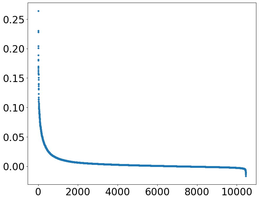
[37]:
def rankplot(df, rank_col = 'I_BV', font_size = 24, figsize = (10, 8), s = 12, save = None):

    '''
    plot the spots according to their values of ´rank_col´

    Parameters
    ---------
    df
        a dataframe containing the spots in rows and ´rank_col´ as a feature value
    rank_col
        rank spots according to their ´rank_col´ values
    font_size
        font size of the tick values of x and y axis
    figsize
        size of the rank plot
    s
        size of the spots
    save
        path to save the rank plot

    '''

    plt.rcParams['font.size'] = font_size
    plt.figure(figsize=figsize)

    t = df[[rank_col]][~df[rank_col].isna()].sort_values(rank_col, ascending = False).reset_index()
    plt.scatter(t.index+1, t[rank_col], s = s)

    if(save != None):
        plt.savefig(save, bbox_inches='tight')
[40]:
import pandas as pd
import matplotlib.pyplot as plt
MoranI_BV = pd.read_csv('Transfer1/MoransI_BV.csv')

rankplot(df = MoranI_BV, rank_col = 'I_BV', save = 'Transfer1/rankplot_BVMI.png')
Calculate location predict scores of genes
This section loads a pre-trained model and uses it to prioritize genes based on their contribution to predicting spatial locations.
[47]:
help(sva.PrioritizeLPG)
Help on function PrioritizeLPG in module SC2Spa.sva:

PrioritizeLPG(adata, Model, sparse=True, polar=True, CT=None, CT_field='MCT', percent=0.5, scale_factor=1000.0, Norm=False)
    Prioritize genes' contribution to location prediction

    Run tl.Self_Mapping first to set Norm as True

    Importance scores will be saved in adata.obs

    Parameters
    ----------
    adata
        Reference anndata object. Gene exprestlon matrix should be the shape of (cell, gene).
        Spatial information should be stored in adata.obsm['spatial']
    Model
        A neural network trained utlng adata.X and adata.obsm['spatial']
    sparse
        if gene exprestlon is saved in sparse format
    CT
        The cell type name used to normalize the importance score.
         it must be one category in `adata.obs[CT_field]`
         This parameter is for normalization
    polar
        Transform cartetlan coordinates to polar coordinates if True.
        This parameter is for normalization
    percent
        The percentage of nodes selected for each layer
    scale_factor
        The factor used to scale the importance scores

    Returns
    -------
Import the
load_modelfunction from Keras.Find common genes between reference (
adata_ref) and query (adata_query) datasets.Create a new AnnData object (
adata) with only the common genes from the reference dataset.Add a ‘gene’ column to
adata.varcontaining the gene names.Load the pre-trained model from the file ‘Model/Cell2Location_snRNAseq2ST_SC2Spa_WD.h5’.
Use the
PrioritizeLPGfunction from thesvamodule to prioritize genes:adata: The AnnData object created in step 3Model: The loaded Keras modelsparse: Set to False (assuming dense matrix)percent: 0.5 (50% of nodes selected for each layer)scale_factor: 1000 (to scale importance scores)Norm: Set to True (normalize the scores)
Ensure that the model file ‘Model/Cell2Location_snRNAseq2ST_SC2Spa_WD.h5’ exists in the specified path.
The
PrioritizeLPGfunction will save importance scores inadata.obs['imp_sumup_norm'].Make sure the
svamodule is imported before running this code.Adjust the
percentandscale_factorparameters if needed for your specific analysis.
[45]:
from keras.models import load_model

JGs = sorted(list(set(adata_ref.var_names).intersection(set(adata_query.var_names))))

adata = adata_ref[:, JGs]
adata.var['gene'] = adata.var.index.tolist()

model = load_model('Model/Cell2Location_snRNAseq2ST_SC2Spa_WD.h5', compile=False)
sva.PrioritizeLPG(adata, Model = model, sparse=False, percent = 0.5, scale_factor = 1e3,
                  Norm = True)
/tmp/ipykernel_2913736/2277315343.py:6: ImplicitModificationWarning: Trying to modify attribute `.var` of view, initializing view as actual.
  adata.var['gene'] = adata.var.index.tolist()
<keras.src.layers.core.dense.Dense object at 0x1554d50a5bd0> :
(4, 2)
<keras.src.layers.core.dense.Dense object at 0x155320bd7d10> :
(16, 4)
<keras.src.layers.core.dense.Dense object at 0x155528d8c110> :
(64, 16)
<keras.src.layers.core.dense.Dense object at 0x1555301c8e10> :
(256, 64)
<keras.src.layers.core.dense.Dense object at 0x1554be0f9290> :
(1024, 256)
<keras.src.layers.core.dense.Dense object at 0x155146a7a6d0> :
(4096, 1024)
<keras.src.layers.core.dense.Dense object at 0x155528897b10> :
(10572, 4096)
[46]:
adata.var.sort_values('imp_sumup_norm', ascending = False).head()
[46]:
| gene_ids | feature_types | genome | n_cells | mt | n_cells_by_counts | mean_counts | pct_dropout_by_counts | total_counts | gene | imp_sumup | imp_sumup_norm | |
|---|---|---|---|---|---|---|---|---|---|---|---|---|
| SPINK8 | ENSMUSG00000050074 | Gene Expression | mm10-3.0.0_premrna | 386 | False | 386 | 0.355682 | 87.060007 | 1061.0 | SPINK8 | 1.504366 | 2.177422 |
| CYP26B1 | ENSMUSG00000063415 | Gene Expression | mm10-3.0.0_premrna | 346 | False | 346 | 0.213208 | 88.400939 | 636.0 | CYP26B1 | 1.211916 | 1.754129 |
| RGS9 | ENSMUSG00000020599 | Gene Expression | mm10-3.0.0_premrna | 578 | False | 578 | 0.357358 | 80.623533 | 1066.0 | RGS9 | 1.080116 | 1.563361 |
| C1QL2 | ENSMUSG00000036907 | Gene Expression | mm10-3.0.0_premrna | 355 | False | 355 | 0.359035 | 88.099229 | 1071.0 | C1QL2 | 1.028882 | 1.489206 |
| SSTR2 | ENSMUSG00000047904 | Gene Expression | mm10-3.0.0_premrna | 642 | False | 642 | 0.345625 | 78.478042 | 1031.0 | SSTR2 | 1.013554 | 1.467020 |
Pearson’s r
[49]:
import seaborn as sns
cmap = sns.cubehelix_palette(n_colors = 32,start = 2, rot=1.5, as_cmap = True)

def VizCus(df, x_name, x_label, y_name, y_label, c_name = None,
           fontsize = 28, vmin= -0.05, vmax = 0.5, s = 14,
           root = 'transfer1/', save = None):

    plt.rcParams['font.size'] = fontsize
    plt.figure(figsize = (12, 8))
    if(c_name == None):
        plt.scatter(df[x_name], df[y_name], s = s)
    elif(vmin!=None):
        plt.scatter(df[x_name], df[y_name], s = s, alpha = 0.7,
                c = df[c_name], vmin = vmin, vmax = vmax, cmap = cmap)
    else:
        plt.scatter(df[x_name], df[y_name], s = s, alpha = 0.7,
                c = df[c_name], cmap = cmap)
    plt.colorbar()
    plt.xlabel(x_label)
    plt.ylabel(y_label)

    if(save != None):
        if not os.path.exists(root):
            os.makedirs(root)
        plt.savefig(root + save + '.png',
                    dpi = 128, bbox_inches='tight')
This section defines a custom visualization function and performs correlation analysis between imputed and reference gene expression data.
[53]:
import numpy as np
from scipy import stats
from IPython.display import clear_output

JCs = sorted(list(set(adata_ref.obs_names).intersection(set(adata_impute.obs_names))))

pearson_JGs = pd.DataFrame(np.zeros((len(JGs), 3)), columns = ['gene', 'pearson_r', 'p'])
pearson_JGs['gene'] = JGs

#Calculate Pearson correlation for each gene
for i, JG in enumerate(JGs):
    print(i)
    t = stats.pearsonr(adata_impute[JCs, JG].X.flatten(), adata_ref[JCs, JG].X.toarray().flatten())
    pearson_JGs.loc[i, 'pearson_r'] = t[0]
    pearson_JGs.loc[i, 'p'] = t[1]
    clear_output(wait = True)

sc.pp.calculate_qc_metrics(adata, percent_top=None, log1p=False, inplace=True)
adata.var['percent_cell'] = adata.var['n_cells_by_counts'] / adata.shape[0]

t = adata.var[['percent_cell', 'imp_sumup_norm']].reset_index()
t.columns =['gene', 'percent_cell', 'imp_sumup_norm']
pearson_JGs = pearson_JGs.merge(t, how = 'left')

pearson_JGs.head(10)
[53]:
| gene | pearson_r | p | percent_cell | imp_sumup_norm | |
|---|---|---|---|---|---|
| 0 | 0610005C13RIK | -0.011918 | 5.638868e-01 | 0.001676 | 0.003440 |
| 1 | 0610009O20RIK | 0.038569 | 6.173370e-02 | 0.227623 | 0.316768 |
| 2 | 0610033M10RIK | -0.001477 | 9.429688e-01 | 0.001676 | 0.004231 |
| 3 | 0610038B21RIK | 0.013289 | 5.199008e-01 | 0.015085 | 0.007029 |
| 4 | 0610039K10RIK | NaN | NaN | 0.001006 | 0.004220 |
| 5 | 0610040B10RIK | -0.008574 | 6.780171e-01 | 0.096882 | 0.138957 |
| 6 | 0610040F04RIK | 0.006385 | 7.571877e-01 | 0.038552 | 0.009026 |
| 7 | 0610040J01RIK | 0.038226 | 6.408569e-02 | 0.060007 | 0.238493 |
| 8 | 1010001B22RIK | -0.007955 | 7.001118e-01 | 0.021120 | 0.007962 |
| 9 | 1010001N08RIK | 0.152428 | 1.136425e-13 | 0.001341 | 0.003459 |
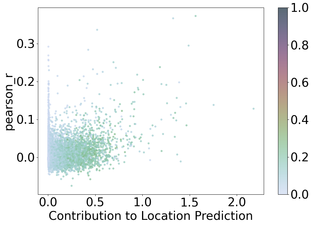
Scatter Plot: Contribution to Location Prediction vs. Pearson Correlation
This scatter plot visualizes the relationship between the contribution to location prediction and the Pearson correlation coefficient for different data points, with points colored based on the percentage of cells a gene is expressed in.
Axes
X-axis: Contribution to Location Prediction
Labeled as “Contribution to Location Prediction,” this axis represents the normalized sum of contributions each data point has on the location prediction model (
imp_sumup_norm). Higher values indicate a greater influence on the prediction.
Y-axis: Pearson r
Labeled as “pearson_r,” this axis represents the Pearson correlation coefficient, which measures the linear correlation between two variables. Values range from -1 to 1, where 1 indicates a perfect positive linear relationship, -1 indicates a perfect negative linear relationship, and 0 indicates no linear relationship.
Color
Color Scale
Points are colored based on the percentage of cells a gene is expressed in (
percent_cell). The color scale ranges from 0 to 1, as indicated by the color bar on the right side.Color bar:
Provides a reference for the percentage of cells, with values ranging from 0 (indicating the gene is expressed in a low percentage of cells) to 1 (indicating the gene is expressed in a high percentage of cells).
Observations
Most data points cluster near the origin, with contributions to location prediction and Pearson r values close to zero.
A few data points exhibit higher contributions to location prediction and higher Pearson r values, indicating stronger linear correlations and greater influence on the prediction model.
The color variation across the plot indicates the distribution of gene expression percentages, with some points representing genes expressed in a higher percentage of cells.
Interpretation
This plot helps identify data points that significantly contribute to the location prediction model and have higher linear correlations with the predicted values.
Points with higher contributions and Pearson r values are of particular interest as they play a crucial role in the model’s performance.
The color of the points provides additional information on the percentage of cells a gene is expressed in, highlighting genes with significant cell representation.
Overall, the scatter plot provides insights into the relationship between the contribution of data points to the location prediction model, their linear correlation, and the percentage of cells a gene is expressed in, aiding in the evaluation and refinement of the model.
[54]:
i = 0

VizCus(pearson_JGs, x_name = 'imp_sumup_norm', x_label = 'Contribution to Location Prediction',
       y_name = 'pearson_r', y_label = 'pearson_r', s = 14, c_name = 'percent_cell',
       vmin = 0, vmax = 1, root = 'Transfer' + str(i+1) + '/',
       save = 'Transfer' + str(i+1) + '_imp_r_pcell.png')
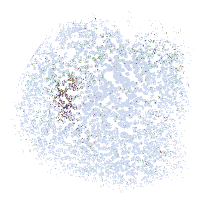
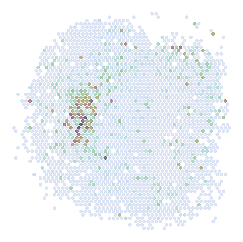
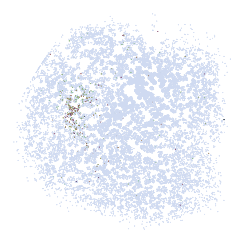
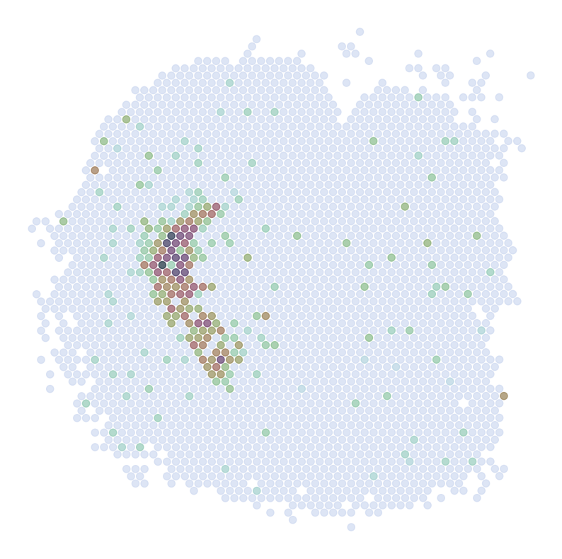
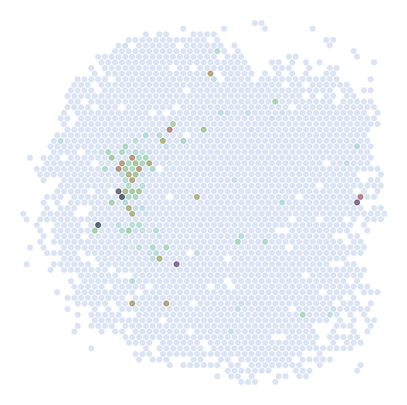
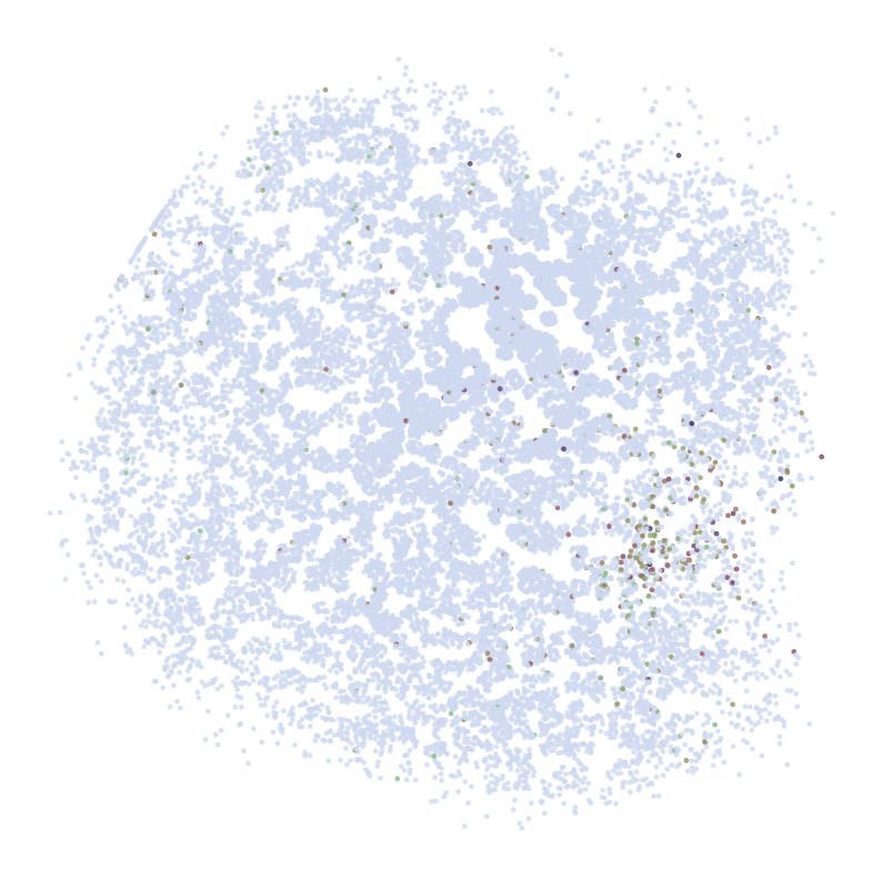
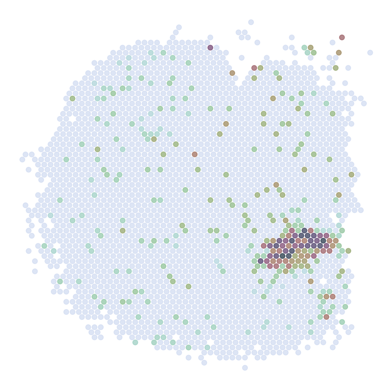
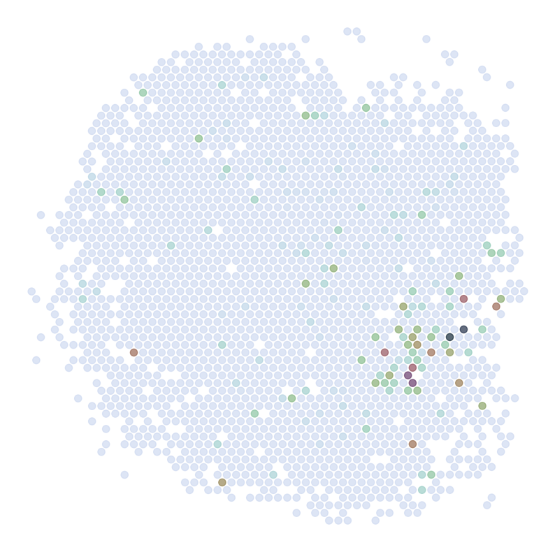
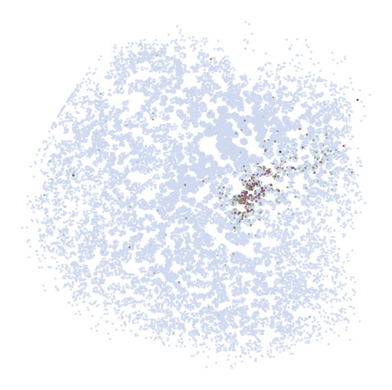
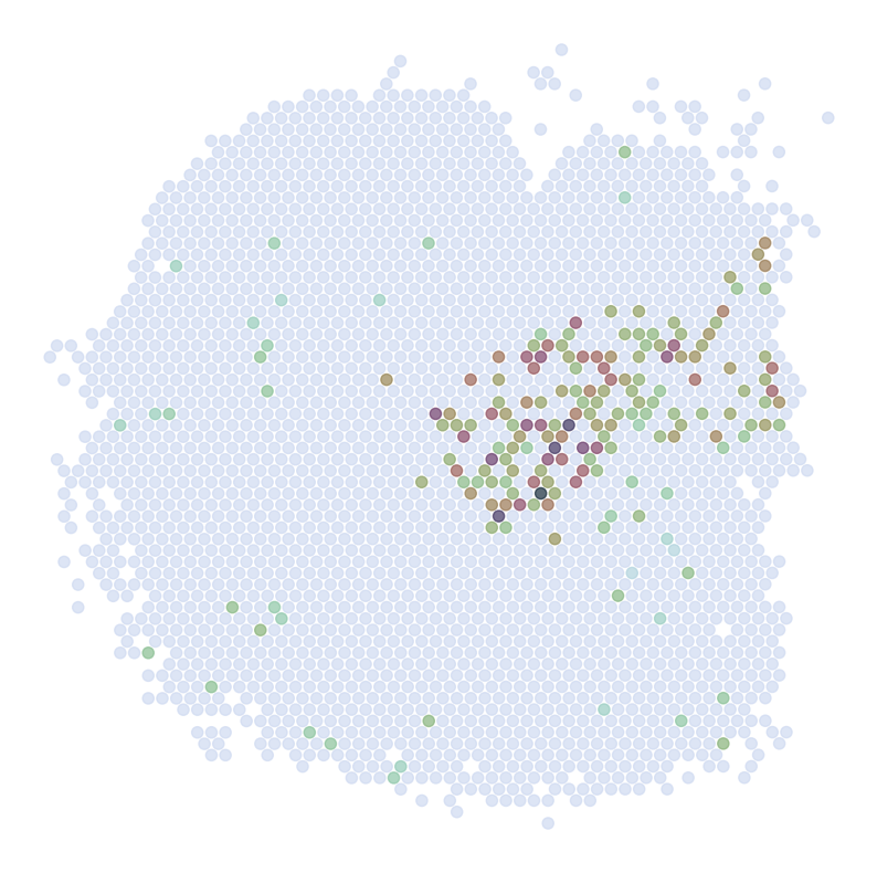
Visualize Top Correlated Genes Across Different Data Types
This code segment visualizes the expression patterns of the top 5 highly correlated genes across single-cell RNA sequencing (scRNAseq), Spatial Transcriptomics (ST), and imputed ST data.
Process:
Select the top 5 genes based on:
Expression in >5% of cells
Highest Pearson correlation between imputed and reference data
For each selected gene:
Visualize gene expression in:
scRNAseq data (using predicted spatial locations)
Original ST data
Imputed ST data (based on location prediction)
Purpose:
This visualization allows for direct comparison of gene expression patterns between the predicted and the original data. It helps validate the imputation process and identify genes that show consistent spatial patterns between the predicted and original data.
Note:
Ensure all required data (adata_query, adata_ref, adata_impute) and the pl module with DrawGenes2 function are properly set up before running this code.
[56]:
GLs = pearson_JGs[pearson_JGs['percent_cell']>0.05].sort_values('pearson_r', ascending = False)['gene'][:5]
pearson_JGs[pearson_JGs['percent_cell']>0.05].sort_values('pearson_r', ascending = False).head(10)
[56]:
| gene | pearson_r | p | percent_cell | imp_sumup_norm | |
|---|---|---|---|---|---|
| 8364 | RGS9 | 0.372766 | 2.900985e-78 | 0.193765 | 1.563361 |
| 986 | ADORA2A | 0.366612 | 1.423300e-75 | 0.082132 | 1.325562 |
| 2757 | DRD2 | 0.336367 | 3.523648e-63 | 0.084814 | 0.520661 |
| 1635 | C1QL2 | 0.294679 | 3.084363e-48 | 0.119008 | 1.489206 |
| 770 | ABHD12B | 0.283610 | 1.155212e-44 | 0.062018 | 0.426028 |
| 8222 | RAB37 | 0.250762 | 5.544544e-35 | 0.133087 | 0.693250 |
| 7653 | PATJ | 0.237858 | 1.517015e-31 | 0.213879 | 1.185487 |
| 2366 | CRLF1 | 0.235978 | 4.623597e-31 | 0.103922 | 0.718446 |
| 6155 | IGFN1 | 0.232128 | 4.396771e-30 | 0.068723 | 0.476038 |
| 6592 | LHX9 | 0.225298 | 2.159814e-28 | 0.078780 | 0.579380 |
[58]:
cmap = sns.cubehelix_palette(n_colors = 32,start = 2, rot=1.5, as_cmap = True)
GLs = pearson_JGs[pearson_JGs['percent_cell']>0.05].sort_values('pearson_r', ascending = False)['gene'][:5]
s1 = 6
s2 = 54
for gene in GLs:
print('*'*32)
print(gene)
print('*'*32)
print('scRNAseq:')
pl.DrawGenes2(adata_query,coords_name = 'spatial_mapping', gene = gene, lim = False, cmap = cmap,
FM = True, CTL = None, c_name = 'simp_name', root = 'Transfer' + str(i+1) + '/FM_Valid2/',
s = s1, title = False, save = 'SC')
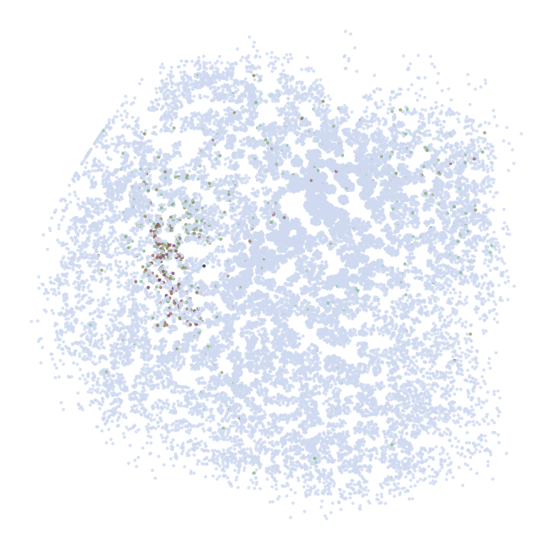
print('ST:')
pl.DrawGenes2(adata_ref, coords_name = 'spatial', gene = gene, lim = False, cmap = cmap,
FM = True, CTL = None, c_name = 'SSV2', root = 'Transfer' + str(i+1) + '/FM_Valid2/',
s = s2, title = False, save = 'ST' + str(i+1))
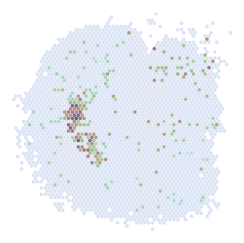
print('Imputed ST:')
pl.DrawGenes2(adata_impute, coords_name = 'spatial', gene = gene, lim = False, cmap = cmap,
FM = True, CTL = None, c_name = 'SSV2', root = 'Transfer' + str(i+1) + '/FM_Valid2/',
s = s2, title = False, save = 'ST' + str(i+1) + '_Impute')
********************************
RGS9
********************************
scRNAseq:
ST:
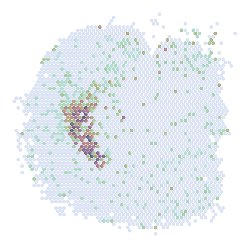
Imputed ST:
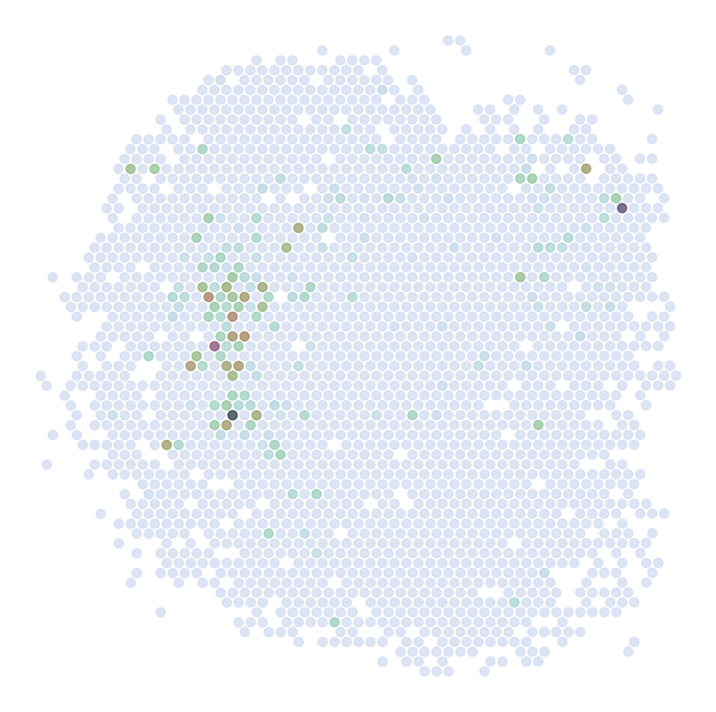
********************************
ADORA2A
********************************
scRNAseq:
ST:
Imputed ST:
********************************
DRD2
********************************
scRNAseq:
ST:
Imputed ST:
********************************
C1QL2
********************************
scRNAseq:
ST:
Imputed ST:
********************************
ABHD12B
********************************
scRNAseq:
ST:
Imputed ST: